Blog - Page 2 of 5 - Fast Reroute

Azure VNet Route Selection

July 1, 2020October 25, 2020 admin

In this blog post, we continue the discovery of virtual networking in Microsoft Azure including in-depth coverage of VNet route tables, subnets, and the process of route selection.

Microsoft Azure Administrator Associate Exam (AZ-104) includes these topics in its blueprint:

configure private and public IP addresses, network routes, network interface, subnets, and virtual network
create and configure VNet peering

We covered basic concepts listed in the first bullet point in the previous article.

This article starts with discussing VNet peering and then dives into additional topics not covered in the first part of the article, such as Azure route tables, network routes, and best route selection process.

Table Of Contents

VNet Peering
Routes and route tables
Azure Best Route Selection Process
Self-Test Questions

VNet Peering

VNet peering connects two VNets together, so resources, such as virtual machines deployed in different networks can communicate with each other. VNet peering provides high-speed, private connectivity using Microsoft backbone.

The peering VNets can be in the same or different regions. If VNets are in the same region, the communication performance between VMs via VNet peering matches the speed and latency of Intra-VNet connectivity.

VNet peering is configured by the provisioning of a peering link in each of the VNets. If VNets are under the same account, the second link can be automatically created. In all other cases, each side needs to be provisioned separately using Resource IDs of the peer VNet. In the lab section, we will demonstrate both options.

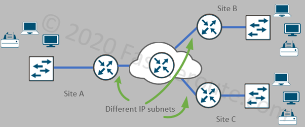
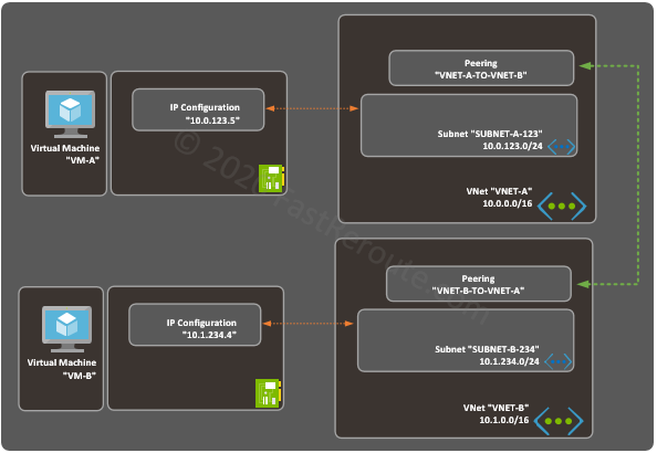
For the practical part of this blog post, we will use the lab topology shown in Figure 1.

Create VNet Peering Step-by-Step

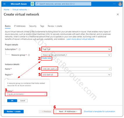
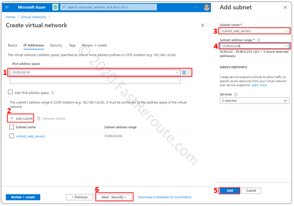
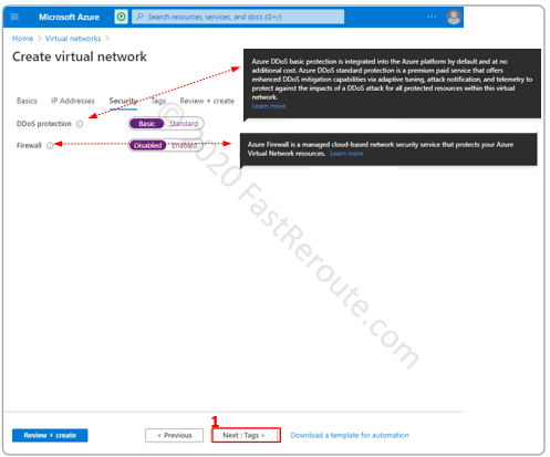
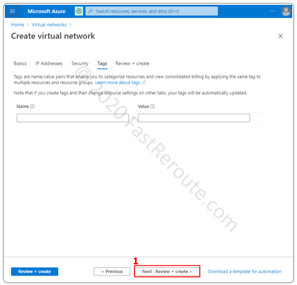
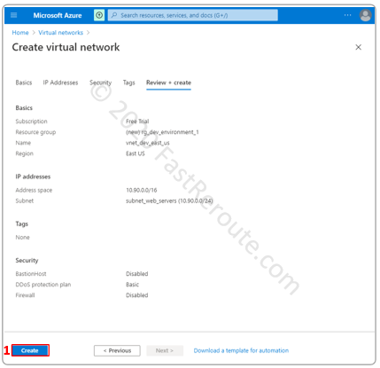
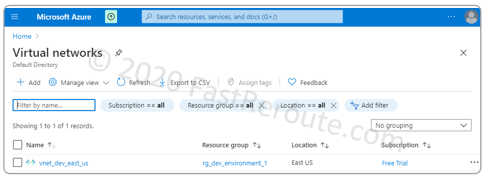
Let’s start this example by creating 2 sets of VNets and subnets. Both VNets will be under the same subscription and in the same region. The detailed procedure on how to create a VNet is available here.

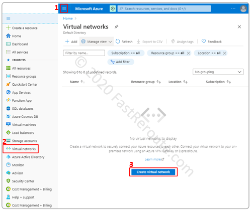
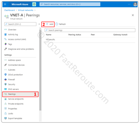
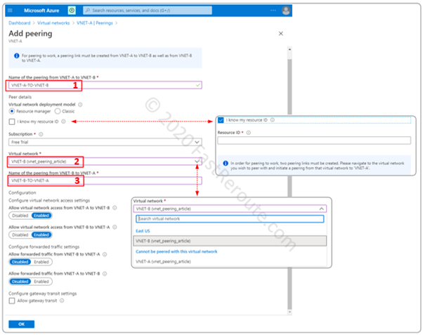
To create a peering open one of the created VNets and select Peerings in the side menu and click Add.

On the “Add peering” page we configured the following settings:

Descriptive name of the peering link on the source VNet side. This is the VNet-A that we selected in the previous screenshot.
Peering virtual network using a drop-down box to select VNET-B, which is accessible from our account.
A descriptive name for the peering that will be automatically added to the target VNet.

To create a peering to VNet that is not in our account, select a checkbox called “I know my resource ID”. Then, instead of Steps 2 and 3, enter the resource ID of the partner VNet. The operation must be repeated in the peering VNet.

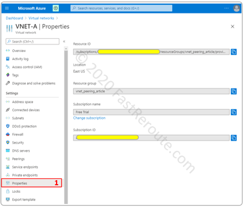
To get the Resource ID of a VNet, navigate to the Properties menu and press the copy to clipboard button next to Resource ID field.

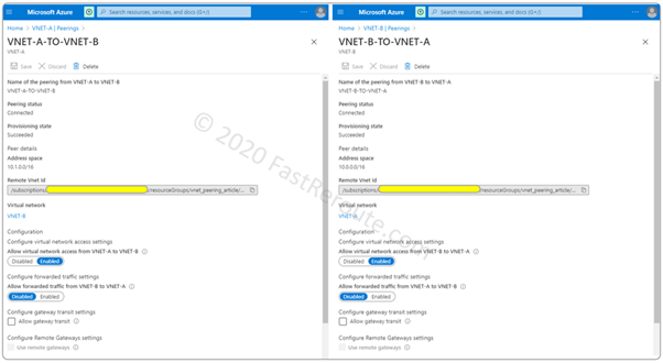
Once peering links are created we can navigate to VNET-A and to VNET-B to validate settings on each side. The screenshot in Figure 5 shows the information on peering status and provisioned state and address space behind the peer. The page also has several configurable parameters.

Virtual network access setting controls if the IP range of a peer is classified as a VirtualNetwork service tag. Both inbound and outbound traffic is allowed between the networks with this tag.

Forwarded traffic, if enabled, permits entry of the traffic that is not originated in the peer VNet. Such traffic usually comes via VPN or ExpressRoute Gateways in the peer VNet. This setting is often used with combination with other two checkboxes:

Allow gateway transit
Use remote gateway

Allow gateway transit allows the peer to use the local VNet’s gateways. Such peering VNet must have “Use remote gateway” checkbox enabled on the peering toward the VNet containing a gateway.

Figure 5. Peering links created in both VNets

Deploy VMs and Testing

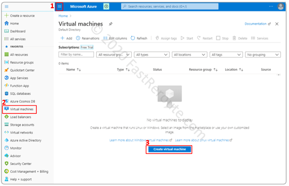
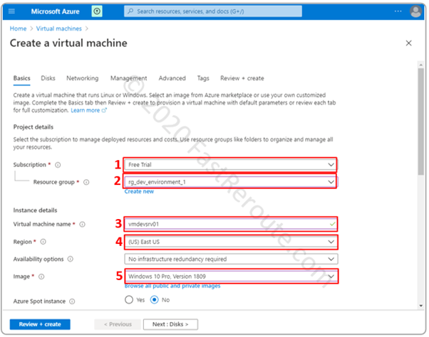
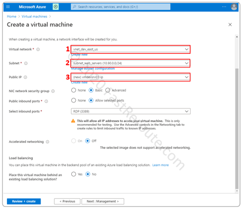
Let’s deploy VMs into corresponding VNets and Subnets according to Figure 1. Use this article for information on how to do it.

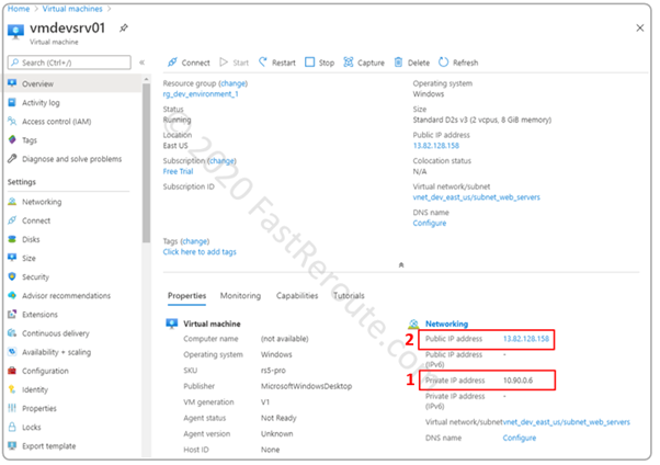
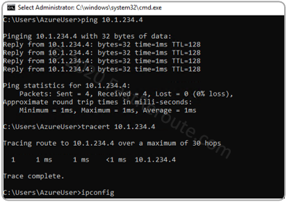
Let’s validate IP address of VM-A by running Windows ipconfig command.

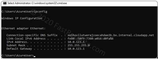
Let’s test that we can ping the VM-B from VM-A. To make this test work we had to disable Windows Firewall on VM-B. In the production environment, it is recommended to keep Windows Firewall enabled, and create a specific rule that allows ICMP through.

Notice that the traceroute doesn’t display any hops between two VMs. This is related to how Azure operates on the back-end. It is different from how packet forwarding works in the traditional data center, where traceroute displays a default gateway as the first hop.

Figure 7. Ping and traceroute testing on VM-A to VM-B

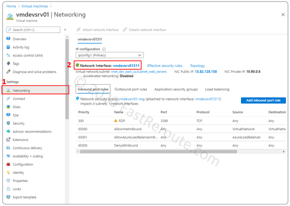
Let’s check Azure VMs security rules and effective routes. Click on the Networking menu of the VM-A. The displayed window has tabs for Inbound and Outbound port rules. They are applied via the Network security group to the network interface, which we will cover in one of the future articles.

In the default configuration, both Inbound and Outbound security rules include a rule (#65000) that allows traffic with the source and destination tagged with VirtualNetwork.

As we discussed earlier, peering’s Access Control Setting checkbox, if enabled, classifies IPs in the peering VNet as part of VirtualNetwork. This effectively allows the traffic to be allowed on Azure level. Guest OS configuration is still required to allow the traffic in.

Figure 8. Inbound and Outbound Rules (Network Security Group)

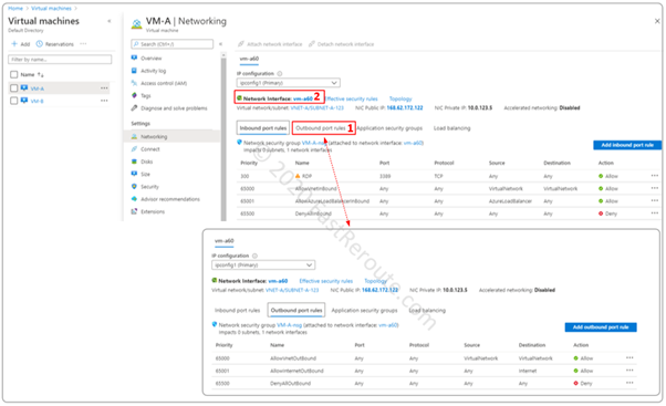
Click on the Network Interface name to proceed to the next step, red rectangle #2 in Figure 8.

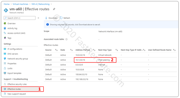
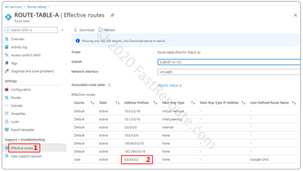
Once the Network interfaces window opens, click on the Effective routes menu, as shown in Figure 9. The routing table has a route to 10.1.0.0/16 with the next hop type of VNet peering.

Figure 9. Effective Routes with VNet Peering route

Routes and route tables

When you create a subnet, it has a default implicit route table associated with it. The Azure portal will not display such tables, and an administrator cannot add custom routes into them. The default route tables contain only system routes, which are automatically added by Azure.

To define a custom route an administrator must create a custom route table and associate it with the subnet. The custom route table will also have automatically added system routes, but these routes can be overridden.

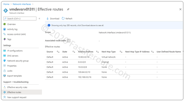
To display routes, use the Effective routes tab of a network adapter, as described in the previous section, and shown in Figure 9. The system routes have Default as their source.

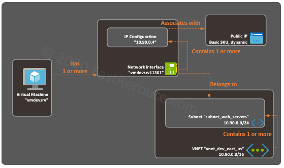
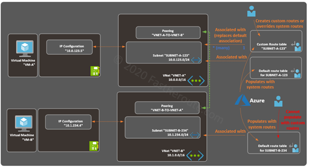
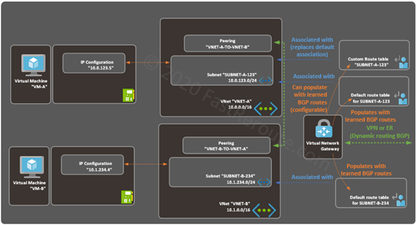
Figure 10 shows a conceptual diagram of relationships between subnets and route tables. Each subnet can have one route table associated with it. A route table, however, can be associated with multiple subnets at the same time.

Figure 10. Azure route table and subnets

(Mandatory) Default System Routes

Azure populates every route table, including the custom route tables, with the following routes.

Route	Next hop type	Comments
Local VNet's address space	Virtual network	In our example, 10.0.0.0/16 for subnets in VNET-A and 10.1.0.0/16 in VNET-B. Note that no subnet-specific routes are created
0.0.0.0/0	Internet	Default route points to Internet. Traffic to Azure public services uses this route, however, it doesn't traverse Internet and stays within Microsoft Azure network
10.0.0.0/8	None	Private RFC 1918 range
100.64.0.0/10	None	Similar to RFC 1918 ranges (reserved for Shared Address Space, see RFC 6598)
192.168.0.0/16	None	Private RFC 1918 range

Table 1. Mandatory Azure System Routes

The default system routes from Table 1 ensure that there is communication within VNet and all traffic is sent to the Internet, with the exception of private address space. Traffic to 3 private ranges is basically discarded.

Interestingly, 172.16.0.0/12 (also part of Private RFC 1918 range) is not among the default null routes. Traffic to this range matches 0.0.0.0/0 and sent to the Internet next hop. It is not routable on the Internet, so it should be discarded somewhere upstream.

(Optional) Default System Routes

Certain routes are only added by Azure into route tables when there is a specific configuration is enabled. For example, in Figure 9 route to a peered VNet was automatically added by Azure. Table 2 lists such routes that can appear in a route table.

Route	Next hop type	Comments
Peered VNet's CIDR block	VNet Peering	Created in route tables of every subnet of a VNet
Public IP addresses of Azure Services	VirtualNetworkServiceEndpoint	Created only in a route table of the subnet that has service endpoint enabled

Table 2. Optional Azure System Routes

Network Gateway Propagated Routes

Figure 11 shows a sample topology with a Virtual Network Gateway.

Virtual Network Gateways provide connectivity to on-premises and external networks connected over VPN or ExpressRoute. The routes to remote networks can (with ExpressRoute gateways – must) be exchanged using Border Gateway Protocol (BGP).

A gateway propagates this information by installing learned routes into route tables. The next-hop type in this case is set to Virtual network gateway.

The propagation is enabled by default, and can be disabled for custom route table using a setting called “Virtual network gateway route propagation”.

Figure 11. Network Gateway Propagated Routes

Custom Routes

In addition to Network Gateway Propagated routes, an administrator can manually create custom ones. Custom routes are preferred in Azure VNet Route Selection Process. We will discuss this in detail in one of the sections below.

To perform this operation a route table must be first created and associated with a subnet. We will demonstrate how to do it in the practical part of this section.

A custom route is identified by its name and requires address prefix and next-hop type to be selected. There are 5 types of next-hops available for Azure custom route:

Virtual network gateway
Virtual network
Internet
Virtual appliance
None

Virtual network gateway next-hop type can be used only for VPN gateways. ExpressRoute must use BGP-based network propagation, so no custom routes can be created to use ExpressRoute Gateway. Notice that there is also no VNet Peering type of the next-hop, which can be created only by Azure. You can, however, create a route that will be pointing to Virtual appliance with Next-hop IP in a peered VNet.

Virtual network next-hop type is used in topologies when you want to make traffic flowing between subnets within a single VNet to go via the virtual appliance. For example, traffic from one subnet to another within a VNet by default is routed via the default system route as discussed in the system routes section. You can override this by selecting the next hop as a virtual appliance. To keep direct traffic flow within the subnet, you can create a custom route with the next hop of the virtual network for the subnet prefix.

Internet next-hop can be used in situations when the default route is overridden and, for example, is sent to the on-premises network to use corporate Internet breakout. To send a subset of traffic via Azure Internet, you create a route for a specific prefix to go via Azure Internet.

Virtual appliance next-hop type requires specifying an IP address of the appliance which will receive traffic. Useful for introducing firewalls and traffic analysis devices.

None next-hop type drops the matching traffic.

Create a Custom Route Table Step-by-Step

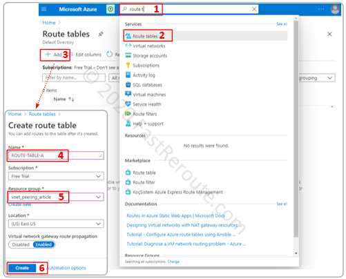
Start typing in “route table” in Microsoft Azure search bar and click on Route tables service. Click on the Add button to create a route table. Fill-in required parameters, including route table name, resource group, and press Create.

Figure 12. Create a new route table - Azure — Figure 12. Create a new route table – Azure

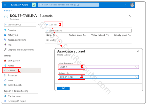
As the next step, we will associate the created route table with Subnet A. Click on the newly created route table and then on the Subnets button on the side menu. Click on the associate button and select the VNet and the Subnet. After this step, SUBNET-A-123 will have a default implicit route table replaced with the custom one.

Figure 13. Associate a route table with subnet - Azure — Figure 13. Associate a route table with the subnet – Azure

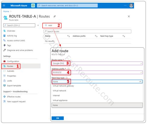
At this stage, the content of the new custom route table will be exactly the same as the routes in the implicit route table. Let’s create a custom route by pressing the Routes button on the side menu and then clicking Add.

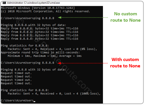
We will create a test route that will discard any packets sent to the Google DNS server IP address of 8.8.8.8/32. To accomplish this, select None as the Next hop type. There are also different types of next-hop types available as we discussed in the theory section.

Figure 14. Create a custom route - Azure — Figure 14. Create a custom route – Azure

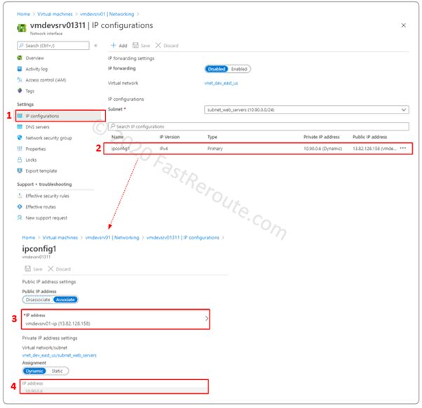
Once we press ok, let’s validate that the route was added and we can also confirm from the virtual machine if the connectivity to 8.8.8.8 no longer works. To validate routes in the custom table, we can use Effective routes accessible via network interface menu or route table menu directly. To display routes via both options, we need to have a network interface attached to a powered-on VM in a subnet that the route table associated with.

Figure 15. Subnet route table validation

The next screenshot shows that connectivity to 8.8.8.8/32 no longer works after we applied a custom route to None.

Figure 16. Connectivity to 8.8.8.8 from VM-A

Azure Best Route Selection Process

The final topic of this article is how the best matching route is selected in Azure.

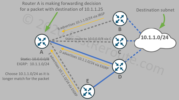
The route selection is intuitive if you follow the rule of not advertising more specific (or the same length) routes that are used in Azure using BGP from an on-premises network or remote VPN networks. If this restriction is maintained, the route selection can be summarized as the following list with the preferred conditions on the top:

1. Longest match

2. User-defined routes

3. BGP-derived

4. System routes

Condition is violated if a network gateway injects via BGP a network that is more specific than (or the same as) VNet address space or a peered VNet prefix. In this case, the routes with the next-hop type of Virtual Network or VNet Peering are preferred over more specific BGP routes. We recommend to design network, so prefixes from Azure VNet address space is not used anywhere else on the network. As a workaround in migration scenarios, remote networks can be network address translated (NAT-ed) to the non-overlapping range.

Let’s consider a few simple examples with 2 Azure VNets with the address prefixes of 10.0.0.0/16 and 10.1.0.0/16. All other networks do not overlap with VNets’ address spaces.

To identify the best route for a specific destination there are several steps, with each minimizing number of candidate routes to select from. Once a single route is left the process stops and this route is used.

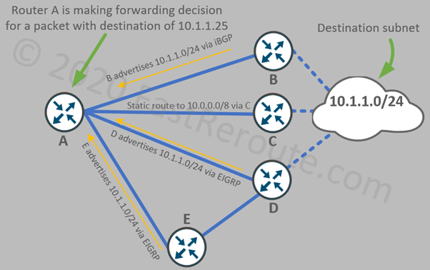
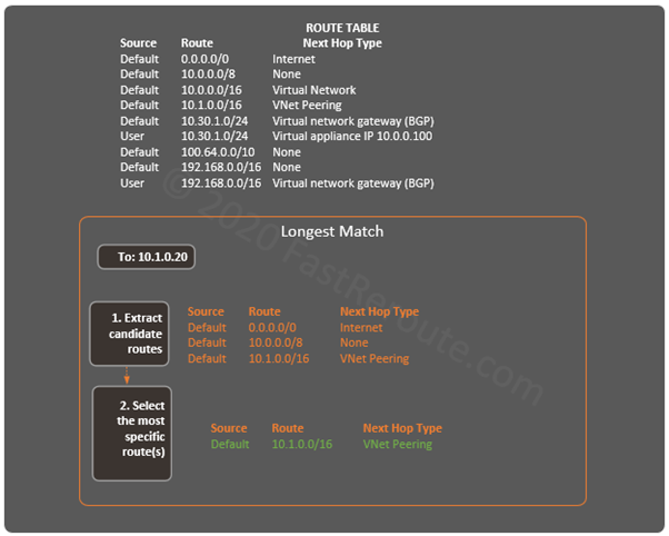
In the diagram below, a packet with the destination of 10.1.0.20 matches 3 routes of different lengths. The most specific route (with the longest prefix length of /16) is selected.

Figure 17. Azure Best Route Selection – Most Specific Route (Longest Match)

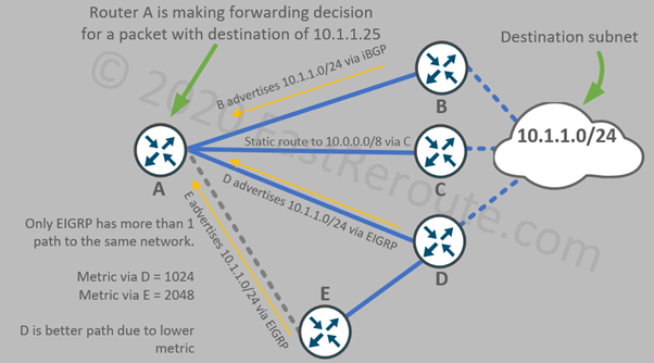
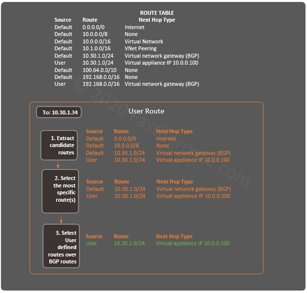
The next example shows a packet with a destination of 10.30.1.34. After selecting all matching candidates, we have 4 routes left. In the second step, we keep only the longest prefix routes (/24). Out of two remaining routes, we know that user-defined routes are more preferred. The single route that points to a virtual appliance with an IP address of 10.0.0.100 is used to forward the traffic.

Figure 18. Azure Best Route Selection – User-defined over BGP

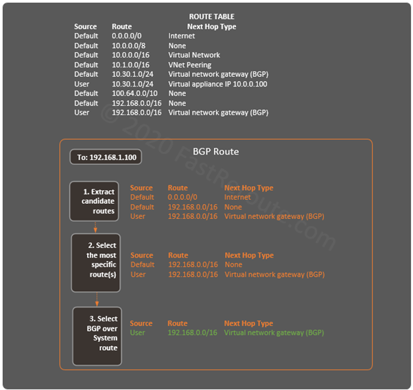
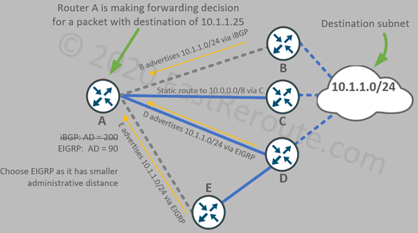
The final example is for a packet with the destination of 192.168.1.100. There are 2 routes left after step 2 with the same length. As BGP routes are preferred over system routes, the packet will be sent to a Virtual network gateway.

Figure 19. Azure Best Route Selection – BGP over System

Self-Test Questions

What is VNet peering?

VNet peering connects two VNets together using high-speed Microsoft backbone. Resources, such as virtual machines deployed in these VNets can communicate with each other.

Is it possible to peer VNets located in different regions?

Yes

What configuration elements are created for VNet peering?

Peering is configured with 2 peering links – one within each VNet.

VNET-A contains a Virtual network gateway that provides connectivity to an external network. You tasked to provision a VNET-B that needs connectivity to the same external network. What configuration is required so VNET-B can use VNET-A's Virtual network gateway?

Create a peering between VNET-A and VNET-B. On VNET-A’s peering link enable the “Allow gateway transit” option. On VNET-B’s peering link enable “Use remote gateway”.

What is relationship between a subnet and a route table in Azure?

A subnet can have a single route table associated with it. By default, a subnet has an implicit default route table associated with it. A route table can be associated with multiple subnets.

What does next-hop type of 'Virtual network' mean in Azure route table?

Represents address space of the VNet. The traffic for the prefixes with this next-hop type will be delivered directly.

Is it possible to create a custom route that uses VNet peering as a next-hop in Azure?

False, VNet peering routes are added by Azure automatically. It is possible, however, to use Virtual appliance as the next hop with IP address in a peered VNet.

When a custom table is associated with a subnet what happens to the Azure system routes?

Azure adds system routes to the custom route tables too. An administrator can override those routes in custom route tables by creating user-defined routes.

How to check routes in a route table in Azure?

An administrator needs a powered-on VM, which has a network interface in the subnet that has the route table associated with it. Navigate to network interface settings page and select the Effective Routes menu.

What are the steps of the best route selection process in Azure. Assume that VNet and its peers have unique address spaces, that doesn't overlap with any other routes?

From the most to the least preferred: Longest match > User-defined routes > BGP-derived routes > System routes

Implement and Manage Virtual Networking

June 22, 2020October 25, 2020 admin

In this blog post, we will explore the basics of Azure Virtual Networking. The target audience of this article is the candidates preparing for the Microsoft Azure Administrator Associate exam (AZ-104).

The exam topic comprises of 2 objectives:

configure private and public IP addresses, network routes, network interface, subnets, and virtual network
create and configure VNet peering

In this post, we will review only basic network configuration, which partially covers the first bullet point. The rest will be covered in the follow-up articles.

Azure Virtual Networking Basics

Figure 1 demonstrates how different components are working together. In the practical section of this blog post, we will go through the process of creating every element shown in this diagram.

Figure 1. Azure Networking Basic Components Interaction

Virtual Network (VNet)

Virtual Network (VNet) is an isolated virtual network environment within the Microsoft Azure cloud. VNETs provide connectivity to other Azure resources, the Internet, and the on-premises network.

A virtual network is scoped to a specific region and subscription. It is identified by a name and has one or many address spaces assigned (IPv4 CIDR block).

Subnets

An administrator can create one or multiple subnets within a single VNet. In the diagram above, a VNet named “vnet_dev_east_us” contains a subnet called “subnet_web_servers”. IP address prefix of a subnet is part of the larger VNet’s prefix.

Virtual Machines and Network Interfaces

Virtual machines can connect to a VNet and a subnet sharing the same region and subscription. Each virtual machine can have one or multiple network interfaces. A network interface is a virtual adapter that connects VM to a subnet.

A network interface is created automatically during VM provisioning. Network interfaces can be detached from VM and it is also possible to create a standalone network interface and attach it to a VM after its creation.

IP Configuration

Both private and public IP addresses are allocated to a network interface using IP configuration. Each IP configuration must have a private IPv4 address and optionally public IPv4 address assigned.

Additional IP configurations provide the ability to add multiple IP addresses to the interface. These IP addresses share the same subnet with the primary IP address.

Private IPs

An IP configuration of a network interface can have a static or a dynamically assigned private IP address in the Azure portal. The dynamic IP address should be used in scenarios when it is acceptable not to have a pre-defined IP address for a VM.

Setting up a static IP address ensures that the VM will be reachable using a pre-defined IP address. The setting in the Azure portal doesn’t enforce dynamic or manual configuration of an IP address within a virtual machine. For example, if the guest Operating System is configured as a DCHP client and Azure portal set to static, the Azure client will still get the address via DHCP. This behavior is similar to a DHCP reservation.

While the type of address assignment can be different, the IP address within the virtual machine must match the one configured in the Azure portal. For example, setting a private IP address statically, that mismatches Azure portal configuration will stop connectivity to that machine.

The First 4 IP addresses (subnet address + first 3 useable addresses) in every subnet are reserved.

Public IPs

Public IP is not configurable within the guest Operating System, which can only see private IP addresses. Azure performs address rewrite, so VM’s private IP address can receive traffic that sent from the Internet to its public IP address, and vice versa – traffic sent to the Internet from a VM is seen as originating from VM’s public IP.

Azure Public IP addresses provide both inbound and outbound connectivity from the Internet to the VM.

Public IPs can be of 2 types – basic SKU and standard SKU (SKU stands for Stock Keeping Unit).

Basic SKU Public IPs can be statically or dynamically allocated. VM with dynamically assigned public IP will release this address when it is stopped.

Standard SKU support high availability with zones and are slightly more expensive than basic SKUs. Standard SKU Public IPs support only static assignments.

Let’s perform simple hands-on configuration to apply the learned concepts to practice.

Create an Azure Virtual Network Step-by-Step

This section shows how to create an Azure Virtual Network step-by-step.

Navigate to Virtual networks administrative page, by selecting it in the left-side menu. In a newly created account, there will be no virtual networks. Click on “Create virtual network” to add one.

Figure 2. Create an Azure Virtual Network – Launching a Configuration Wizard

We will choose the only available subscription in our account, which is Free Trial. A subscription can contain resource groups; which have the purpose of grouping together resources with the same lifecycle. Let’s create a new resource group and name it rg_dev_environment_1.

Type-in a name for the VNet and region in which it will exist.

Figure 3. Create an Azure Virtual Network Wizard – Basic Parameters

We will use an IPv4 address space of 10.90.0.0/16 and create a new subnet. It must be within VNet’s IP address space. In the example below, we’ve added subnet 10.90.0.0/24 and named it “subnet_web_servers”.

As shown in the screenshot below, it is possible to allocate multiple IPv4 address spaces to a virtual network.

Figure 4. Create an Azure Virtual Network Wizard – IP Addresses and Subnets

The next step provides an option to enable security features, such as DDoS protection and Firewall. For the purpose of this demonstration, we will keep the default settings.

Figure 5. Create an Azure Virtual Network Wizard – Security

Tagging provides the ability to add custom metadata to different resources, which can be used for management and billing purposes. We will proceed to the next step without applying any tags.

Figure 6. Create an Azure Virtual Network Wizard – Tags

The final step of the wizard provides summary information. Click on Create button to add the network.

Figure 7. Create an Azure Virtual Network Wizard – Review

The Virtual networks list is now populated with the new VNet we’ve created.

Attaching a VM to Azure Virtual Network

This section demonstrates how to connect a virtual machine to a subnet in a virtual network while creating a new VM. Only network-relevant details will be shown and discussed.

To add a new virtual machine, open the side menu, and select Virtual Machines. Click on the “Create virtual machine” button.

Figure 9. Create an Azure Virtual Machine – Launching a Configuration Wizard

In the “Basics” dialogue window define general VM parameters, such as the subscription, resource group, and the virtual machine name. The regions of a VM should match the region of VNet, otherwise, the subnet will not be available for selection in the Networking step.

Figure 10. Create an Azure Virtual Machine – Basics

We moved straight to the Network configuration step skipping Disks configuration.

Figure 11 shows the configuration section related to networking. The virtual network drop-down menu will contain only VNets that are in the same region as the VM. We also select a subnet in which VM’s interface will be placed.

Figure 11. Create an Azure Virtual Machine - Networking — Figure 11. Create an Azure Virtual Machine – Networking

All remaining settings are left unchanged and VM has been created.

Reviewing the VM Configuration

After a few minutes VM is provisioned and we can check its settings. As Figure 12 shows, the machine was assigned a private IP address of 10.90.0.6 with the public IP address of 13.82.128.158.

Figure 12. Review an Azure Virtual Machine – Overview

The networking submenu of the virtual machine displays network interface and Network Security Group (NSG) settings. Let’s click on the interface to see its configuration.

Figure 13. Azure Virtual Machine – Networking Settings

Network adapter settings include IP configurations. During the machine provisioning process, we could only access the primary IP configuration. This menu allows for creating additional IP configurations, which are similar to secondary IP addresses. It can be useful for adding multiple IP addresses, for example, for a web server with multiple websites, each available on different IP addresses.

This configuration menu also exposes the IP forwarding setting, which allows network adapter to accept packets that don’t have destination IP addresses matching any of the interface’s addresses. This configuration is required for devices that perform routing functions, such as 3^rd party firewalls or intrusion protection systems.

Figure 14. Azure Network Adapter – IP Configuration Settings

Inbound Internet Connectivity

Public IP addresses provide inbound connectivity to a virtual machine over the Internet.

We can now use Remote Desktop Connection (RDP) client to access this virtual machine. To launch RDP client on Windows 10 machine start typing “Remote Desktop” and select the built-in application.

Type in the public IP address of the VM and press Connect in RDP client. Use credentials provided during VM provisioning (default username is AzureUser).

Outbound Internet Connectivity

After connecting to a VM’s remote desktop, let’s open a web browser to test outbound Internet connectivity and check the public IP address that the VM uses.

To perform this testing, type in “what is my IP” request into the Google search bar. As shown in Figure 15, the outbound IP address matches the one we saw in the previous example.

Figure 15. Checking Azure Virtual Machine Public IP Address

Validating Routing Table in Azure portal

VNet uses the default route table to decide where to send Internet traffic when VM tries to connect to external resources. Subnets and route tables interaction will be a subject of one of the next blog posts, however, for now, we can check the effective routes as seen from VM’s network adapter point of view.

To do it navigate to Network interfaces menu, select Network adapter attached to the virtual machine, and click on Effective routes.

Figure 16. Checking Azure Virtual Machine Effective Routes

As shown in the screenshot, we can see that the default route has a Next Hop Type of Internet.

Self-Test Questions

Can a single VNet be used to provide connectivity for virtual machine that belong to multiple Microsoft Azure customers?

No, Virtual Network (VNet) is an isolated virtual network environment.

Can a single VNet span multiple regions in Azure?

No, a VNet is scoped to a specific region.

What is the relationship between a VNet and a subnet?

VNet contains one or more subnets.

Can a network interface exist separately from a virtual machine?

Yes, it is possible to create a network interface and later attach it to a VM

What is IP Configuration?

IP Configuration is a property of a network adapter that defines a single private IP address and, optionally, a single public IP address

When an administrator configures public IP address in Azure portal, does he need to configure it within guest Operating System?

No, Azure performs address rewrite, so a VM can see only private addresses at the network layer. Application payload still may contain public IP addresses, so in certain cases, a VM might need to know its public IP address.

Interpret JSON Encoded Data

June 14, 2020October 25, 2020 admin

In this blog post, we will discuss the JavaScript Object Notation (JSON) data format. The target audience is CCNA and CCNP candidates preparing for the exams.

The content provides fundamental overview of the following topics:

CCNA exam

6.7 Interpret JSON encoded data

CCNP ENCOR exam

6.2 Construct valid JSON encoded file

JSON Overview

JSON is an open standard text-based file format to store and exchange serialized data. Serialization is the process of converting an object into a format that can be stored or transported to later recreate it.

JSON was originally derived from JavaScript, however, many other programming languages can interpret and generate JSON data. Figure 1 shows how JSON components fit together.

JSON text can represent one of the following values (orange and blue circles):

String
Number
Literal name (false, true, null)
Array
Object

Figure 1. JSON Values, Objects and Arrays

JSON simple values

Strings, numbers, and literals

The simple values can represent some text or number and cannot contain other values. For example, below are examples of valid JSON texts:

Listing 1

"I'm a JSON"
100
true
null

As per RFC 8259, JSON text can be represented by any serialized value. Some specifications of JSON require that valid JSON text must be an object or an array.

Note that the string values must be enclosed in quotation marks.

JSON structured data values

Structural characters

JSON values that represent structured data (blue circles) created using 6 structural characters listed below:

Square brackets [] – beginning and end of an array
Curly brackets {} – beginning and end of an object
Colon : – Name separator
Comma , – Value separator

JSON allows the use of whitespaces, such as spaces, tabs, and new lines to format the text for readability. Contrasted to Python, indentation is used only for readability.

Array

An array contains zero or multiple ordered elements. Elements don’t have to be of the same type.

Listing 2

[ "abc", 23, null ]

Object

An object contains zero or multiple members, separated by commas. Each member is in the name: value format. Name must be unique within an object.

Listing 3

{ 
    "address": "192.168.8.1", 
    "mask": "255.255.255.255" 
}

Nested Objects and Arrays

Arrays and objects can contain both simple values, other arrays, and other objects.

For instance, below is the object, as we can see it starts with an opening curly brace. The object contains 2 members with name tags of “primary_address” and “secondary_address”. Each of the member’s value is another object that consists of 2 more members, named “address” and “mask”.

Listing 4

{ 
    "primary_address": 
    {
        "address": "192.168.8.1", 
        "mask": "255.255.255.255"
    },
    "secondary_address": 
    {
        "address": "192.168.9.1", 
        "mask": "255.255.255.255"
    },
}

Let’s create an array that will contain 2 objects representing addresses. The opening square bracket starts the definition of an array. Then we wrap each of the members from the previous example into curly brackets to create an object, as array stores elements – not members consisting of name: value pairs.

Listing 5

[ 
    {
        "primary_address": 
        {
            "address": "192.168.8.1", 
            "mask": "255.255.255.255"
        }
    },
        "secondary_address": 
        {
            "address": "192.168.9.1", 
            "mask": "255.255.255.255"
        },
    }
]

How to interpret JSON encoded data

In one of the previous blog posts dedicated to REST API, we’ve programmatically extracted a JSON representation of an interface from the IOS-XE router. This listing below shows several router’s interfaces, so we can have some arrays in the example.

Listing 6

{
  "Cisco-IOS-XE-native:interface": {
    "GigabitEthernet": [
      {
        "name": "1",
        "ip": {
          "address": {
            "primary": {
              "address": "192.168.7.4",
              "mask": "255.255.255.0"
            }
          }
        },
        "mop": {
          "enabled": false,
          "sysid": false
        },
        "Cisco-IOS-XE-ethernet:negotiation": {
          "auto": true
        }
      },
      {
        "name": "2",
        "shutdown": [
          null
        ],
        "mop": {
          "enabled": false,
          "sysid": false
        },
        "Cisco-IOS-XE-ethernet:negotiation": {
          "auto": true
        }
      }
    ]
  }
}

Let’s interpret this document. Figure 2 shows the structure of the JSON code from the example above.

The top-level object (#1) has a single member with the name of “Cisco-IOS-XE-native:interface”. This member’s value is another object (#2).

The object #2 also has a single member named “GigabitEthernet”, whose value is an array (#3).

Array contains 2 elements – object #4 and object #5.

Object #4 has 4 members, with the following names:

“name”
“ip”
“mop”
“Cisco-IOS-XE-ethernet:negotiation”

Member called “name” has a string value of “1”. The next member named “ip” has an object (#6) as a value. Object #6 has a single member with the name of “address” having another object (#7) as a value.

The pattern of finding array elements and object members should be apparent by now.

Figure 2. Cisco IOS-XE RESTCONF JSON interpretation example

How to construct JSON encoded data

Online Tools

The easiest way to create a JSON encoded data is to use one of the available online JSON editors. For example, one is available via this URL. It automatically checks JSON file syntax, which can be useful to find a missing bracket. The other feature of this tool is the ability to auto-format code into a compact format or full format (with line breaks and indentation, as shown in the previous example).

The screenshot of the tool with JSON text from the previous example is shown below.

Python Collections Overview

To continue with the following examples, we recommend checking this article (URL) for a brief quick start and Python installation instructions.

Let’s discuss several Python fundamental topics before proceeding with the practical examples.

Data Structures: lists and dictionaries

Lists and dictionaries are examples of collections in Python. Python’s JSON module maps lists to JSON arrays, and dictionaries to JSON objects.

The syntax is identical between matching pairs of data structures, as shown in Figure 4.

Figure 4. Mapping of JSON structured data to Python collections

The listing below shows an example of a list and a dictionary definition in Python.

A list is defined in Python using square brackets. Python uses None instead of null literal in JSON.

The dictionary is wrapped with curly brackets and has familiar from JSON example syntax. JSON’s name tag (value just before the colon) corresponds to a dictionary key in Python. It is followed by a colon and a value, which is in our example a string.

Listing 7

sample_list = [ "abc", 23, None ]
sample_dictionary = { "address": "192.168.8.1", "mask": "255.255.255.255" }

Let start interactive Python prompt to demonstrate how to work with lists and dictionaries.

Listing 8

c:\PythonExamples>python
Python 3.8.3 (tags/v3.8.3:6f8c832, May 13 2020, 22:20:19) [MSC v.1925 32 bit (Intel)] on win32
Type "help", "copyright", "credits" or "license" for more information.
>>> sample_list = [ "abc", 23, None ]
>>> sample_dictionary = { "address": "192.168.8.1", "mask": "255.255.255.255" }

Both lists and dictionaries can be passed to print() method, which will display their string representation.

Listing 9

>>> print(sample_list)
['abc', 23, None]
>>> print(sample_dictionary)
{'address': '192.168.8.1', 'mask': '255.255.255.255'}

We can access individual elements in a list using their index position.

Listing 10

>>> print(sample_list[0])
abc
>>> print(sample_list[1])
23

To extract values for a specific dictionary key, we can use the key’s name as an index.

Listing 11

>>> print(sample_dictionary["address"])
192.168.8.1
>>> print(sample_dictionary["mask"])
255.255.255.255

Working with files

We will save and read JSON files to and from a file saved on the disk in the next examples.

To open a file for read access in Python the following code is used:

Listing 12

with open("json_test.json","r") as json_file:
    … some code that makes use of json_file

To open the same file for write access, use “w” instead of “r” as a parameter for the open() function. Use of keyword “with” ensures that the file is properly closed after the use.

Decoding JSON in Python example

Python module called json provides JSON encoding and decoding capabilities. There are 2 methods performing these functions:

dumps – Python data structure to JSON text
loads – JSON text into Python data structure

Let’s create a text file containing JSON text from Listing 6 and save it as json_ios_xe.json.

As the next step, we will create a file named json_example.py that will have the following Python code in it.

Listing 13

import json

with open("json_ios_xe_interfaces.json", "r") as json_file:
    json_file_content = json_file.read()
decoded_json = json.loads(json_file_content)

print(decoded_json)
print()
print(type(decoded_json))

Line #1 imports json module, so we can use its feature in our code.

The code in line #3 opens our file for read-only access. The access to the file content is provided via json_file variable. The code in line #4 reads-in content of the file into a string variable.

Line #5 uses json.loads() function to read the string representation of JSON text. The returned value is assigned to the decoded_json variable. As the JSON text is a JSON object, the decoded_json object will be a Python dictionary.

Line #7 prints the Python dictionary, followed by an empty line created by line #8. Finally, line #9 prints out the type of decoded_json object, so we can validate that it is in fact a Python dictionary.

Let’s run the code and see the result.

Listing 14

c:\PythonExamples>python json_example.py
{'Cisco-IOS-XE-native:interface': {'GigabitEthernet': [{'name': '1', 'ip': {'address': {'primary': {'address': '192.168.7.4', 'mask': '255.255.255.0'}}}, 'mop': {'enabled': False, 'sysid': False}, 'Cisco-IOS-XE-ethernet:negotiation': {'auto': True}}, {'name': '2', 'shutdown': [None], 'mop': {'enabled': False, 'sysid': False}, 'Cisco-IOS-XE-ethernet:negotiation': {'auto': True}}]}}

<class 'dict'>

Encoding to JSON in Python example

In this example, we will use the dictionary created in the previous example, change the IP address to “192.168.7.5” and will encode it as another JSON file.

The first task is to identify the full path to the IP address. We have several nested layers of hierarchy within the outer-most dictionary. To access inner dictionaries and lists we will append [<index_or_key_name>] to the parent identifier.

Full path to value of ‘address’ key will be:

Listing 15

decoded_json['Cisco-IOS-XE-native:interface']['GigabitEthernet'][0]['ip']['address']['primary']['address']

In the example above the index of [0] is used, as the ‘GigabitEthernet’ key has the value of a list and we are interested in the first element.

Below is the full listing of a program code that changes the IP address and saves it as a new JSON file on the disk.

Listing 16

import json

with open("json_ios_xe.json", "r") as json_file:
    json_file_content = json_file.read()

decoded_json = json.loads(json_file_content)

decoded_json['Cisco-IOS-XE-native:interface']['GigabitEthernet'][0]['ip']['address']['primary']['address'] = \
    "192.168.7.5"

encoded_json_compact = json.dumps(decoded_json)
encoded_json_indented = json.dumps(decoded_json, indent = 4)

with open("json_ios_xe_compact.json", "w") as json_file:
    json_file.write(encoded_json_compact)

with open("json_ios_xe_indented.json", "w") as json_file:
    json_file.write(encoded_json_indented)

Line #8 sets the value to a new IP address. Lines #11 and #12 create a string containing JSON text, it passes our modified dictionary called decoded_json to json.dumps() function. The example demonstrates that the named parameter called “indent” can be passed to the dumps() method to perform the formatting of the JSON file.

Line #15 and #18 saving the resulted text to files on the disk.

Let’s run the code and see the result.

Listing 17

c:\PythonExamples>python json_example.py

Two new files are created in c:\PythonExamples folder, as shown in the screenshot below.

Figure 5. JSON text decoded by Python's json.dumps() — Figure 5. JSON text decoded by Python’s json.dumps()

Self-Test Questions

List 6 types of value types that JSON text can represent?

String, number, Boolean (false, true), null, array, and object.

Describe JSON array and the process of defining one.

A JSON array contains ordered elements and defined using square brackets. For example, [ “abc”, 23, null ]

Describe JSON object and the process of defining one.

A JSON object contains members separated by a comma. Each member has a name and value separated by a colon. It is defined using curly brackets. For example, { “address”: “192.168.8.1”, “mask”: “255.255.255.255” }

Name Python types that are mapped to JSON's array and object

Python’s list maps to JSON array, and Python’s dictionary maps to a JSON object

What Python's module is responsible for encoding and decoding of JSON-formatted data?

json module. To decode use json.loads() and to encode – json.dumps().

Interpret Basic Python Components and Scripts

June 8, 2020October 25, 2020 admin

In this blog post, we will provide an introduction to Python components and scripts in the context of Cisco certification. We will show how to get started with Python and explain the most commonly used elements of Python scripts – variables, functions, program flow, conditional logic, and “for” loops.

The content aims to help CCNP/CCIE Enterprise track candidates to prepare for the ENCOR exam, which includes the following topic:

6.1 Interpret basic Python components and scripts

Many CCNP tracks have automation sections that assume some knowledge of Python. DevNet track expects more extensive knowledge in Python.

Python Installation

Python is an interpreted language, which means that the code of a program is not pre-compiled into an executable that contains machine instructions. Python code can be opened and edited with any text editor. Python programs have a .py extension.

To run a Python code an interpreter is required. It reads the code and converts it into machine instructions.

Python is available for different platforms. Python 3.x is the recommended version and we will use it in our examples.

To download Python installation files navigate to this URL. Start the installer.

We use Windows 10 in our examples. Enable the checkbox “Add Python 3.x to PATH” and press Install Now.

Start Windows CLI utility by starting typing “Command Prompt”. Once started type in the following command to confirm that Python interpreter is available.

Microsoft Windows [Version 10.0.18362.836]
(c) 2019 Microsoft Corporation. All rights reserved.

C:\PythonExamples>python --version
Python 3.8.3

Keep the command prompt window opened.

Hello World!

We will start with a simple “Hello World!” example.

Open a text editor, such as Notepad, and type-in the following code:

print("Hello World!")

The example uses a built-in print() function that displays a message on the screen.

Save the file as hello_world.py in a folder on your computer. To run the program, we will pass the full file name to python interpreter:

C:\PythonExamples>python c:\PythonExamples\hello_world.py
Hello World!

Variables

A variable stores some value, which can be accessed in the code by using its name. In Python, variables are not declared and can be used by assigning a value to them.

Let’s add a few more lines to the hello_world file. The new code creates a line number variable that is changed after each use. First two times it was statically set to 2 and 3, and in the line, before the last, we’ve just incremented its value by 1. The print function is being provided with 2 arguments – descriptive text and the line number variable.

print("Hello World!")
line_number = 2
print("This is the line number", line_number)
line_number = 3
print("This is the line number", line_number)
line_number = line_number + 1
print("This is the line number", line_number)

When the program is launched the following output is displayed on the screen.

C:\PythonExamples>python c:\PythonExamples\hello_world.py
Hello World!
This is the line number 2
This is the line number 3
This is the line number 4

Functions

A function minimizes the amount of duplicate code. It can also provide better structure and improve the readability of program code, by wrapping related logic under the function definition, which can be called by a descriptive name from other places of the program.

Let’s adjust our program to demonstrate the use of functions.

def line_number_printer(number):
    print("This is the line number", number)

def calculate_next_line_number(previous_number):
    return previous_number + 1

print("Hello World!")
line_number = 2
line_number_printer(line_number)
line_number = calculate_next_line_number(line_number)
line_number_printer(line_number)
line_number = calculate_next_line_number(line_number)
line_number_printer(line_number)

The program produces exactly the same output as the code in the previous example.

We have introduced 2 functions:

line_number_printer(number)
calculate_next_line_number(previous_number)

Figure 2 shows how the functions are defined and used in the example above. Not all lines from the example are shown for brevity.

Let’s go through the diagram and discuss each element:

A function’s definition must precede its use. The code within the definition is not executed unless it is called.
Function definition starts with a keyword “def”.
The function name should be in lower case with underscore used as a word separator. Python’s style guide is called PEP 8. It explains different elements of style, such as the naming convention and how the code must be formatted (https://www.python.org/dev/peps/pep-0008).
A function can accept a value as an input in the form of parameter. Variable name in parentheses stores value supplied when the function was called. This variable is available for use within the function body.
The line containing function definition ends with a colon showing that function statements will follow in the next lines.
The code statements within a function are indented. PEP 8 recommends the use of spaces for indentation instead of tabs. Also, 4 spaces should separate each indentation level.
A function can be invoked to perform some action without returning any values to the caller. It can also return a value; such as a result of a calculation or a success code back to the caller. To create such a function, a statement starting with keyword return is used. When this statement is encountered, function execution stops.

Conditional Logic

Conditional logic statements allow us to perform certain actions based on an evaluation result of a condition. Let’s modify our example, so the line_number_print function displays different strings depending on whether the number is odd or even. The listing below shows the modifications made, the remaining code is not changed.

def line_number_printer(number):
    if number % 2 == 0:
        print("This is the line number", number, "and it is even")
    else:
        print("This is the line number", number, "and it is odd")

When the program is launched the following output is displayed on the screen.

C:\PythonExamples\>python c:\PythonExamples\hello_world.py
Hello World!
This is the line number 2 and it is even
This is the line number 3 and it is odd
This is the line number 4 and it is even

Figure 3 shows how conditional logic is used in the example above.

Figure 3. Python Conditional Logic Example

Let’s go through the diagram and discuss each element:

“if” keyword is followed by a logical test that can be either True or False.
If the test is evaluated as True, the statement (or multiple statements) under the “if” section is executed.
As with the functions, the body of “if” or “else” sections comprises of indented statements.
If the test is evaluated as False, the statement (or multiple statements) under the “else” section is executed.

for Loops

The “for” loops can be used to apply an action to each element of a collection. For example, we can store a list of switch interfaces in a list. To check the status of each of these interfaces we can use the “for” loop to iterate through the list and then run a command against each of the interfaces.

Let’s rewrite our program using “for” loops to automatically assign line numbers.

The listing below shows the complete code, as we removed the line calculation function and multiple calls to print function.

def line_number_printer(number):
    if number % 2 == 0:
        print("This is the line number", number, "and it is even")
    else:
        print("This is the line number", number, "and it is odd")

print("Hello World!")
for line_number in range(2, 5):
    line_number_printer(line_number)

When the program is launched the same output is displayed on the screen.

C:\PythonExamples>python c:\PythonExamples\hello_world.py
Hello World!
This is the line number 2 and it is even
This is the line number 3 and it is odd
This is the line number 4 and it is even

Figure 4 shows how “for” loop is used in the example above.

Figure 4. Python "for" loop Example — Figure 4. Python “for” loop Example

Let’s go through the diagram and discuss each element:

“for” keyword is followed by a variable name that will be changing its value on each pass.
“in” keyword is followed by a list of values that will be assigned one at a time to the “for” variable on each iteration.
Statements that perform actual work during each cycle are indented under the “for” loop.

Not shown in the example, “break” keyword stops loop processing and continues with the code following the loop. Similarly, the “continue” keyword stops the current pass processing, but in contrast to “break”, it starts the next cycle of the loop.

Self-Test Tasks:

Task 1

Write a function that accepts a number and prints it out followed by “is the number passed as a parameter”.

Task 2

Write a function that accepts a number and prints out “Greater than 10” or “Less or equal than 10” depending on the number that was provided. The greater operator is “>” and less or equal is “<=”.

Task 3

Write a “for” loop that iterates over a list of interfaces Ethernet1/1, Ethernet1/2, and Ethernet1/3 and prints out the output below. To supply interfaces for “for” loop, use a list [ “Ethernet1/1”, “Ethernet1/2”, “Ethernet1/3” ]

interface Ethernet1/1
 description Added by Automation Script
 no shutdown
interface Ethernet1/2
 description Added by Automation Script
 no shutdown
interface Ethernet1/3
 description Added by Automation Script
 no shutdown

Self-Test Answers:

Task 1

def print_number(number):
    print(number, "is the number passed as a parameter")

Task 2

def compare_number_to_ten(number):
    if number > 10:
        print("Greater than 10")
    else:
        print("Less or equal than 10")

Task 3

for interface_name in [ "Ethernet1/1", "Ethernet1/2", "Ethernet1/3" ]:
    print("interface", interface_name)
    print(" description Added by Automation Script")
    print(" no shutdown")

vSphere 7.0 Editions

June 2, 2020June 2, 2020 admin

Editions and Packaging

vSphere 7 is available from April 2020. It is available in the same editions as vSphere 6.7 except for vSphere Platinum edition. As with vSphere 6.7, a support and subscription contract (SNS) is required. See our article on 6.7 editions here.

vSphere Standard and vSphere Enterprise Plus are the two main editions. Standard edition offers a base set of features, and Enterprise Plus extends the feature set with advanced capabilities.

VMware announced the end of availability (EOA) for vSphere Platinum Edition. AppDefense SAAS is now available as a standalone offering. See the details here.

vSphere 7 introduces add-on for Kubernetes, which allows deploying containerized applications. It is available as part of the VMware Cloud Foundation.

Licensing is CPU count-based. However, VMware had an update for the per-CPU pricing model in March 2020. After this update, CPUs with core count exceeding 32 require an additional license. Detailed information is available here.

As in previous editions, different types of packages and licensing types are available:

vSphere Desktop. It can be used only for Virtual Desktop Infrastructure (VDI) deployments with either VMware Horizon View or third-party connection brokers.
vSphere Acceleration Kits. These are bundles of vSphere licenses for 6 or 8 CPUs and a license for vCenter Server. The kits are convenience packages for purchasing. The actual licenses and software contracts can be used and renewed independently.
vSphere Essentials Kits. These kits have enforceable limits of 3 hosts with 2 CPU each and a license for a single instance of vCenter Server for Essentials. In comparison to vSphere Acceleration Kits, Essentials Kits cannot be combined with other editions or decoupled.
vSphere Remote Office Branch Office. This type of packaging limits the number of VMs available for deployment to 25 and targets remote branches.
vSphere Scale-Out. This package is sold in packs of 8 CPUs for high-performance computing (HPC) and big data.

The following table lists feature set as available at the time of writing (June 2020). Check the following document for up-to-date information (URL).

Certain features may not be listed for specific packaging in VMware datasheets. To eliminate ambiguity, we’ve marked such features as “Not listed explicitly”.

Feature	Essentials	Essentials Plus	ROBO Standard	ROBO Advanced	ROBO Enterprise	Scale-Out	Standard	Enterprise Plus
vSphere Hypervisor	•	•	•	•	•	•	•	•
vMotion		•	•	•	•	•	•	•
VMware vCenter Hybrid Linked Mode	Not listed explicitly	Not listed explicitly	Not listed explicitly	Not listed explicitly	Not listed explicitly	Not listed explicitly	vCenter Server Standard	vCenter Server Standard
vSphere Virtual Symmetric Multiprocessing (SMP)	Not listed explicitly	Not listed explicitly	•	•	•	Not listed explicitly	•	•
vSphere High Availability (HA)		•	•	•	•	Not listed explicitly	•	•
Storage vMotion	Not listed explicitly	Not listed explicitly	•	•	•	•	•	•
Fault Tolerance	Not listed explicitly	Not listed explicitly	2 vCPU	4 vCPU	4 vCPU	Not listed explicitly	2 vCPU	8 vCPU
VMware vShield Endpoint		•	•	•	•	•	•	•
vSphere Replication		•	•	•	•	Not listed explicitly	•	•
Support for 4K native storage	Not listed explicitly	Not listed explicitly	Not listed explicitly	Not listed explicitly	Not listed explicitly	Not listed explicitly	•	•
vSphere Quick Boot		•	•	•	•	•	•	•
vCenter High Availability	vCenter Server Essentials	vCenter Server Essentials	vCenter Server Foundation	vCenter Server Foundation	vCenter Server Foundation	vCenter Server Standard	vCenter Server Standard	vCenter Server Standard
vCenter Backup and Restore	vCenter Server Essentials	vCenter Server Essentials	vCenter Server Foundation	vCenter Server Foundation	vCenter Server Foundation	vCenter Server Standard	vCenter Server Standard	vCenter Server Standard
vCenter Server Appliance Migration Tool	vCenter Server Essentials	vCenter Server Essentials	vCenter Server Foundation	vCenter Server Foundation	vCenter Server Foundation	vCenter Server Standard	vCenter Server Standard	vCenter Server Standard
TPM 2.0 support and virtual TPM	Not listed explicitly	Not listed explicitly	Not listed explicitly	Not listed explicitly	Not listed explicitly	Not listed explicitly	•	•
FIPS 140-2 compliance and TLS 1.2 support		•	•	•	•	•	•	•
Support for Microsoft virtualization-based security (VBS)		•	•	•	•	•	•	•
Per-VM Enhanced vMotion Compatibility	Not listed explicitly	Not listed explicitly	Not listed explicitly	Not listed explicitly	Not listed explicitly	Not listed explicitly	•	•
VMware Instant Clone	Not listed explicitly	Not listed explicitly	Not listed explicitly	Not listed explicitly	Not listed explicitly	Not listed explicitly	•	•
Identity federation with Active Directory Federation Services (ADFS)	Not listed explicitly	Not listed explicitly	•	•	•	•	•	•
Content Library	Not listed explicitly	Not listed explicitly	•	•	•	•	•	•
APIs for Storage Awareness	Not listed explicitly	Not listed explicitly	•	•	•	•	•	•
APIs for Array Integration, Multipathing	Not listed explicitly	Not listed explicitly	Not listed explicitly	Not listed explicitly	Not listed explicitly	•	•	•
Virtual Volumes and Storage-Policy Based Management	Not listed explicitly	Not listed explicitly	•	•	•	•	•	•
Next-generation infrastructure image management		•	•	•	•	•	•	•
Cross-vCenter and Long Distance vMotion	Not listed explicitly	Not listed explicitly	Not listed explicitly	Not listed explicitly	Not listed explicitly	Not listed explicitly		•
VM encryption	Not listed explicitly	Not listed explicitly			•	Not listed explicitly		•
Distributed Switch	Not listed explicitly	Not listed explicitly		•	•	•		•
Host Profiles and Auto Deploy	Not listed explicitly	Not listed explicitly		•	•	•		•
Distributed Resource Scheduler (DRS)	Not listed explicitly	Not listed explicitly			• (limited)	Not listed explicitly		•
Distributed Power Management (DPM)	Not listed explicitly	Not listed explicitly	Not listed explicitly	Not listed explicitly	Not listed explicitly	Not listed explicitly		•
Storage DRS	Not listed explicitly	Not listed explicitly	Not listed explicitly	Not listed explicitly	Not listed explicitly	Not listed explicitly		•
I/O Controls (Network and Storage) and SR-IOV	Not listed explicitly	Not listed explicitly	Not listed explicitly	Not listed explicitly	Not listed explicitly	•		•
vSphere Trust Authority	Not listed explicitly	Not listed explicitly	Not listed explicitly	Not listed explicitly	Not listed explicitly	Not listed explicitly		•
vSphere Persistent Memory	Not listed explicitly	Not listed explicitly	Not listed explicitly	Not listed explicitly	Not listed explicitly	Not listed explicitly		•
NVIDIA GRID vGPU	Not listed explicitly	Not listed explicitly	Not listed explicitly	Not listed explicitly	Not listed explicitly	Not listed explicitly		•
Proactive HA	Not listed explicitly	Not listed explicitly	Not listed explicitly	Not listed explicitly	Not listed explicitly	Not listed explicitly		•
Predictive DRS	Not listed explicitly	Not listed explicitly	Not listed explicitly	Not listed explicitly	Not listed explicitly	Not listed explicitly		•
Accelerated graphics for VMs	Not listed explicitly	Not listed explicitly	Not listed explicitly	Not listed explicitly	Not listed explicitly	Not listed explicitly		•
Dynamic vSphere DirectPath I/O™	Not listed explicitly	Not listed explicitly	Not listed explicitly	Not listed explicitly	Not listed explicitly	Not listed explicitly		•
vCenter Server Profile	Not listed explicitly	Not listed explicitly	Not listed explicitly	Not listed explicitly	Not listed explicitly	Not listed explicitly		vCenter Server Standard
vCenter Server update planner	Not listed explicitly	Not listed explicitly	Not listed explicitly	Not listed explicitly	Not listed explicitly	Not listed explicitly		•
Bitfusion	Not listed explicitly	Not listed explicitly	Not listed explicitly	Not listed explicitly	Not listed explicitly	Not listed explicitly		2 GPU

vCenter Server is available in 3 editions:

vCenter Server for Essentials (up to 3 hosts; can manage only Essentials and Essentials Plus)
vCenter Server Foundations (up to 4 hosts; can manage Standard, Enterprise Plus and vCloud Suite)
vCenter Server Standard (unlimited hosts; can manage Standard, Enterprise Plus and vCloud Suite)

Feature and Scaling Comparison by Version

To check the full and the latest information, follow this URL.

Feature	vSphere 6.5	vSphere 6.7	vSphere 7
Kubernetes, VMware Tanzu Runtime and Hybrid Infrastructure Services			• (VMware Cloud Foundation)
vMotion (storage, cross-vSwitch, cross-vCenter, long-distance, cross-cloud hot and cold)	•	•	•
Content Library	•	•	•
Per-VM enhanced vMotion compatibility		•	•
DRS, Storage DRS	•	•	•
Enhanced DRS			•
Network-aware DRS		•	•
Network and Storage I/O Control	•	•	•
Assignable hardware support for vGPU and DirectPath I/O initial placement			•
Fault Tolerance	4 vCPU	8 vCPU	8vCPU
Replication, HA VM component protection, Proactive HA, vCenter HA, Orchestrated HA Restart	•	•	•
Virtual Volumes, Storage Policy-based Management, NFS 4.1 Support, Automated UNMAP	•	•	•
Support for 4K native storage		•	•
Multifactor Authentication, vSphere security hardening and compliance, VM encryption, Secure boot, Audit quality logging	•	•	•
TPM 2.0, virtual TPM 2.0, support for Microsoft VBS, FIPS 140-2 Validated		•	•
vSphere Trust Authority, Identity federation with ADFS			•
VMware Instant Clone, NVIDIA vGPU	•	•	•
vSphere Integrated OpenStack, vSphere Integrated Containers	•	•	•
vMotion support for NVIDIA vGPU, vSphere Persistent Memory, support for memory mapping for 1GB page size		•	•
Support for RoCE v2, iSCSI extension for RDMA (iSER), Support for RDMA InfiniBand		•	•
vCenter Server Appliance, Certificate management, Migration to vCenter Server Appliance	•	•	•
Enhanced Linked Mode, vCenter Server Hybrid Linked Mode, vCenter Server backup and restore	•	•	•
HTML5-based vSphere Client, REST-based API for vCenter Server Management	•	•	•
Single reboot upgrades, vSphere Quick Boot, vCenter Server Appliance backup with built-in scheduler and retention		•	•
vSphere Lifecycle Manager, vCenter Server update planner, vCenter Server Profiles			•

Table 2. vSphere 6.5, 6.7 and 7.0 Feature Comparison

vSphere 7 supports a higher number of hosts per cluster and a higher number of hosts for linked vCenter servers. Table 3 captures scaling limits for different editions.

Scale Metric	vSphere 6.5	vSphere 6.7	vSphere 7
Hosts per cluster	64	64	96
VMs per cluster	8,000	8,000	8,000
Hosts per VMWare vCenter Server	2,000	2,000	2,000
Power-on VMs per vCenter Server	25,000	25,000	30,000
Hosts for 15 linked vCenter Servers	5,000	5,000	15,000
CPUs per host	576	768	768
RAM per host	12TB	16TB	16TB
VMs per host	1,024	1,024	1,024
vCPUs per VM	128	128	128
vRAM per VM	6TB	6TB	6TB
Non-volatile memory per host		1TB	1TB
Non-volatile memory per VM		1TB	1TB

Table 3. vSphere 6.5, 6.7 and 7.0 Scaling Limits Comparison

Describe characteristics of REST-based APIs

May 30, 2020October 25, 2020 admin

In this blog post, we will discuss REST-based APIs. We will also demonstrate how to use such APIs with step-by-step scenarios using a Cisco virtual router running on the ESXi platform.

This article aims to help CCNA candidates in preparing for the following exam topic:

6.5 Describe characteristics of REST-based APIs (CRUD, HTTP verbs, and data encoding)

APIs and Representational State Transfer (REST)

Application Programming Interface (API)

API of an application or a service specifies how other applications can access and change its information. For example, a service may expect certain parameters to be specified when a client application makes a request. The service generates some output as a response, which is also part of API.

A network device manufacture develops and maintains API. CCNA candidates should understand how to use APIs from the client perspective. Automation scripts and software use APIs that network devices expose.

Command-Line Interface (CLI) cannot be classified as API. It provides means to change how a device operates, but its primary purpose is to interact with a user, i.e. not with another program. CLI, however, can be used in automation scripts, which interactively send and parse command output.

SNMP operation fits the definition of API. However, it didn’t receive wide adoption in network automation and is mostly used in read-only monitoring.

Cisco devices and controllers expose RESTful APIs, i.e. APIs that meet specific architectural criteria. We will discuss this type of API in the following section.

RESTful API

REST defines a set of architectural guidelines that were defined by Roy Fielding in his dissertation.

REST is not a protocol and doesn’t provide specific implementation details. For example, it doesn’t mandate the use of HTTP, which is, however, is most often used and often associated with REST APIs.

REST defines a set of constraints that must be met for a web service to be considered RESTful. The full list of constraints is:

Must have client-server architecture.
RESTful services must have a uniform interface.
The client must track the state of the session and send request containing all information required to process such a request. The server must not store user session context information.
The server must state whether information can be cached on the client.
The system must have a hierarchical layered design.
The server can send executable code to a client to extend its functionality.

RESTful API constraints provide multiple benefits for an application and are important for an API designer to follow. However, for a network engineer, the main areas of focus are centered around how to access and change information behind API.

REST Resources and Representation

In REST API a resource is any type of information that can have a name. For example, a network interface or an access list can be used as resources in API.

A resource is identified with a Uniform Resource Identifier (URI). Type of URI that specifies a location and access protocol of a resource is called Unified Resource Locator (URL). When a client sends a request to REST API, it must include a resource identifier. For example, if HTTP is used as protocol, the URL of https://fastreroute.com/category/ccna consists of the URI scheme of HTTPS, followed by colon, authority “//”, hostname – fastreroute.com, and resource identifier (or path) – /category/ccna.

Representation of a resource is a self-describing state of a resource at a specific moment. The server provides a representation of a resource to the client, which can perform different operations on the resource. For example, the representation of the resource identified with the URL in the previous paragraph is an HTML page that contains all CCNA posts of the blog. REST APIs can return representation as a serialized object, for example, in (JavaScript Object Notation) JSON format.

CRUD and HTTP Verbs

CRUD stands for 4 generic types of operations that can be applied to data:

Create
Read
Update
Delete

HTTP request methods, also called verbs, can be mapped to CRUD operations. For example, in an HTTP-based RESTful API, a client can change the parameters of a network interface by using the HTTP PATCH method. We will show how it can be done in the example section.

HTTP GET method corresponds to Read operation. The server responds with a representation of a resource identified by URI.

HTTP POST verb Creates a child or subordinate to resource specified in URI.

HTTP PUT maps to both Update and Create operations. If a resource specified in the PUT request exists on the server, it should be replaced with the one in the request. If the resource doesn’t exist, PUT can create it.

HTTP PATCH verb can also perform the Update operation. PATCH contains instructions on how to update a resource, while PUT contains a modified copy of a resource.

HTTP DELETE maps to Delete operation.

REST API Example: CSR1000v

Let’s apply concepts from the previous section to practice. The next few sections will show how to perform each of CRUD operations with REST-like API provided by Cisco IOS-XE routers.

This API is based on RESTCONF. It can return the representation of resources in XML or JSON formats. RESTCONF uses YANG, which is modeling language describing a router’s configuration and operation states.

Both RESTCONF and YANG are described in RFCs:

8040 RESTCONF Protocol (https://tools.ietf.org/html/rfc8040)
6020 YANG – A Data Modeling Language for the Network Configuration Protocol NETCONF (https://tools.ietf.org/html/rfc6020)

IOS-XE Configuration for RESTCONF

In our example, we will generate API requests to a CSR1000v IOS-XE router running on ESXi.

Our router runs IOS-XE version 16.9.5 with the following configuration applied:

interface GigabitEthernet1
 ip address 192.168.7.4 255.255.255.0
 no shutdown
aaa new-model
aaa authentication login default local
aaa authorization exec default local

username admin secret ciscocisco
username admin privilege 15
enable secret ciscocisco

ip http server
ip http authentication local
ip http secure-server
restconf

Refer for details to the Cisco configuration guide, which is available via this URL.

Postman Client Setup

We will use free tier features of software called Postman (https://www.postman.com/).

Postman helps with testing and discovery of API prior to writing automation programs. The automation scripts can be written using programming languages, such as Python with requests library.

Download the software for the platform of your choice. We use the Windows version of Postman in the next examples and the screenshots.

Start Postman and disable SSL certificate validation, as we are going to use the router’s IP address and self-signed certificate in our examples:

Figure 1. Postman - Disable SSL Certificate Verification — Figure 1. Postman – Disable SSL Certificate Verification

Read with HTTP GET

In the first example, we will send a simple GET request to obtain a list of interfaces of the router.

The next figure shows the sequence of steps creating the request in Postman that returns the list of interfaces of the router. The username and password values must match ones configured on the router.

In this example, the URL of https://192.168.7.4/restconf/data/Cisco-IOS-XE-native:native/interface/ consists of the following components:

https – URI scheme and protocol
// – authority
192.168.7.4 – hostname or IP address of the router
/restconf/data/Cisco-IOS-XE-native:native/interface/ – path or resource ID

Figure 3. Postman –GET Request Parameters

The result of the request is shown in the next screenshot. The server replied back with a 200 OK message and a representation of its interfaces in XML format.

Figure 4. Postman – Read list of the Router's Interfaces in XML Format — Figure 4. Postman – Read list of the Router’s Interfaces in XML Format

To switch to JSON we can adjust the request by modifying Headers as shown in Figure 5. Accept key is set to value of application/yang-data+json. The response looks very similar to the one in Figure 4, as both XML and JSON represent the same resource – a list of interfaces of the router.

Figure 5. Postman – Read list of the Router's Interfaces in JSON Format — Figure 5. Postman – Read list of the Router’s Interfaces in JSON Format

Create new interface with HTTP POST

As the next step, let’s create a new loopback interface using the HTTP POST verb. Figure 6 demonstrates a message exchange between the client using URI representing a list of interfaces and the POST method containing the JSON representation of the new loopback interface. The server returns HTTP response with the code of 201 (created).

Figure 6. Cisco IOS-XE REST API Create an Interface with HTTP POST

Figure 7 shows Postman configuration for this request.

Figure 7. Postman - Create an Interface with HTTP POST — Figure 7. Postman – Create an Interface with HTTP POST

The listing below shows JSON representation of the interface:

{
  "Cisco-IOS-XE-native:Loopback": {
    "name": "1",
    "description": "Test",
    "ip": {
      "address": {
        "primary": {
          "address": "192.168.8.1",
          "mask": "255.255.255.255"
        }
      }
    }
  }
}

The router has its configuration updated with new Loopback1 interface:

ROUTER#show run interface Loopback1
!
interface Loopback1
 description Test
 ip address 192.168.8.1 255.255.255.255
!

Update interface description with HTTP PATCH

In this example, we will create a query that sets the GigabitEthernet1 interface’s description. Figure 8 shows the message exchange between the PC and the router. URI includes interface name, as PATCH is used to apply partial updates to an existing interface.

Figure 8. REST API Update with HTTP PATCH

Postman query configuration steps are shown in Figure 9. Note that authorization settings must be set in the same way as done in the HTTP GET example.

Figure 9. Postman – Updating Interface Description using HTTP PATCH

The listing below shows JSON representation of the description change:

{
  "Cisco-IOS-XE-native:GigabitEthernet": {
    "description": "Very Important Interface",
  }
}

The router has its configuration updated with a description:

ROUTER#show run interface GigabitEthernet1
!
interface GigabitEthernet1
 description Very Important Interface
 ip address 192.168.7.4 255.255.255.0
 negotiation auto
 no mop enabled
 no mop sysid
!

Delete interface description with HTTP DELETE

The final example will delete the Loopback interface using the HTTP DELETE verb. Figure 8 shows the message exchange, which identifies the resource that we want to delete.

Figure 8. REST API Delete with HTTP DELETE

Figure 9 shows configuration parameters in Postman.

Figure 9. Postman – Deleting Interface with HTTP DELETE

And the listing below demonstrates that the interface doesn’t exist anymore:

Router#show run interface Loopback1
                                  ^
% Invalid input detected at '^' marker.

Self-Test Questions

What is REST and RESTful API?

REpresentational State Transfer (REST) is an architectural style that defines a set of constraints to create APIs. RESTful API is an API that meets all the constraints.

Does RESTful API have to be HTTP-based?

No, REST doesn’t mandate the use of any specific protocols.

What is the difference between Resource and Representation in REST?

A resource is a named piece of information, while a representation of the resource is a description of the resource at a specific moment.

Map CRUD operations to HTTP verbs

Create – POST or PUT.
Read – GET.
Update – PATCH or PUT (by replace).
Delete – DELETE

Explain the role of DHCP and DNS within the network

May 18, 2020October 25, 2020 admin

In this blog post, we will cover the role of 2 important services – DHCP and DNS. The CCNA exam includes the following topics that we will explore in detail:

4.3 Explain the role of DHCP and DNS within the network

4.6 Configure and verify DHCP client and relay

Domain Name System

Domain Name System (DNS) is a naming protocol for hosts and services on the Internet. It is also a client-server application that maintains and provides access to DNS records. Many Internet services, such as web browsing and email delivery, rely on DNS service.

In addition to its role of naming hosts on the Internet, DNS is also often used by organizations to support their internal applications. For example, Microsoft Active Directory is a directory service that requires DNS to store its records. In such scenarios, the internal records are not exposed to the Internet.

Domains and FQDNs

Hosts are uniquely identified by their Fully Qualified Domain Name (FQDN). For example, server1.sales.fastreroute.com is a fully qualified domain name of a server. The name consists of 2 parts separated by a dot:

Hostname portion, or server1
Domain portion, or sales.fastreroute.com

The domain component is hierarchical, with the parent domains specified on the right side. In the example above, domain .com is a parent domain of fastreroute.com, which in turn is a parent domain of sales.fastreroute.com.

To understand domain hierarchy, a file system can be used as an analogy, in which folders are replaced with domains and files with hosts. Domains can contain sub-domains or hostnames, in the same way as a file-system folder can contain subfolders or files.

Name Servers

Name server functionality can be implemented as an operating system component, an application, or Software-As-A-Service (SAAS). For example, BIND is one of the most popular DNS servers on the Internet and is available on Unix-like operating systems. Windows platforms have a DNS server built-in into the server operating system.

Public cloud providers offer managed DNS service, for example, AWS offers Route53, which can provide advanced features beyond traditional DNS servers. Cisco routers can be configured to act as a DNS server too. We will provide an example of how to set it up in this blog post.

A name server can act as an authoritative server or name resolver, or both at the same time. The authoritative server role focuses on storing naming information in DNS zones. The resolver role is about providing requested information after receiving a query from a client. We will discuss these roles in detail in the next two sections.

Authoritative Name Servers and Zones

An authoritative name server stores a DNS zone for a specific domain subtree and doesn’t rely on querying other name servers for entries in this zone. A domain hierarchy defines a logical structure of a namespace, while zones are actual files or databases storing the DNS data.

The very top zone in the hierarchy of public DNS is called the root zone. It contains pointers on how to find information about domains such as .com, .net, and different country codes. These domains are called Top-Level Domains (TLDs).

The root zone is serviced by 13 groups of DNS servers, which are also called root hints. Each group contains geographically distributed servers that share the same anycast IP address and allocated a letter of the alphabet as hostname, in the root-server.net domain. The location of these servers on the world map can be checked here, scroll down to see members within each cluster, and their location.

When an organization registers a domain name, for example, fastreroute.com, the parent domain (.com) delegates administrative control over fastreroute.com and all domains under it to the organization. If no further delegation is done, then the zone fastreroute.com will store all entries in the domain and all subdomains under it.

Administrators of fastreroute.com can delegate control of a subdomain sales.fastreroute.com to the sales department. A different set of DNS servers can host the zone for sales.fastreroute.com and all subdomains under it, such as us.sales.fastreroute.com.

If we continue the analogy with the file system, delegation is similar to creating a link or shortcut that will redirect users to another file server. This server, in turn, can create shortcuts to other file servers and so on.

Name Resolvers and Query Types

Name resolution is the process of a DNS client sending a query and DNS server replying to it. The most commonly used type of request is to resolve hostnames to IP addresses. Some name servers can perform only name resolution functionality and do not host any zones, i.e. not being authoritative for any domain namespaces.

There are 2 modes that name resolvers can operate in – recursive and iterative. A recursive server can perform additional queries to another server if it doesn’t have the required information locally. Recursive name resolvers can also cache answers, so the subsequent queries can be serviced using a local cache. An iterative resolver, instead of doing all the queries on the client behalf, can return an address of another name server for the client to query directly.

Record types

DNS stores information in domain zones using several types of records. SOA record contains authoritative zone information, administrative contacts, and different timers. NS record contains pointers to authoritative DNS servers.

“A” record maps a hostname to an IPv4 address. AAAA record is the IPv6 version of A record. PTR record stores reversed A record, so one can resolve a hostname by using an IP address.

CNAME record keeps hostname to hostname mapping and also often called alias record. MX record is used to specify the SMTP mail server for a domain. TXT record stores a piece of text information.

Check this article on Wikipedia with the full list of DNS record types.

Cisco Routers and Switches as a DNS Client

Cisco devices can be configured as a DNS client. The device has multiple system services such as, Smart Licensing and NTP servers, that use hostnames and need to figure out the IP addresses. Hostname and domain name is also used to create RSA keys for services, such as the SSH server.

The following configuration commands configure DNS client functionality:

hostname edgerouter1
ip name-server 8.8.8.8 8.8.4.4
ip domain name fastreroute.com

In this example, the router will have FQDN of edgerouter1.fastreroute.com. It will use two Google’s name servers in the specified order and it will also append suffix fastreroute.com if only a hostname is specified in various commands.

To display name server information, validate cache and enable debugging, use the following 3 commands:

show ip dns servers
show hosts
debug ip domain

Cisco Routers and Switches as DNS Server

It is possible to configure Cisco routers to provide DNS server functionality. To enable it use the following command:

ip dns server

By default, the server will use name servers configured on the router, as shown in the earlier example, to perform query forwarding. It is possible to create conditional forwarding patterns useful when you might want to use internal DNS servers for some queries and ISP’s DNS servers for Internet access at the remote branch. The configuration guide on the Cisco website provides more information for such a configuration.

It is also possible to create static entries that can be useful for different testing scenarios:

ip host test.local.lab 1.2.3.4

In this example, the router will reply with the IP address of 1.2.3.4 to clients that are trying to resolve “test.local.lab” via the Cisco router.

Dynamic Host Configuration Protocol (DHCP)

A host needs an IP address to communicate on the network. An address can be assigned to a device via manual configuration or dynamic assignment. Administrators manually configure IP addresses on servers and network devices that expect static IP addresses. DHCP server dynamically assigns IP addresses to workstations and client devices, as they don’t expect inbound connections and manual configuration would be time-consuming and unpractical.

DHCP Client-Server Communication

When a DHCP client starts up, it broadcasts a discover message looking for a DHCP server. As the client doesn’t have an IP address during bootstrap, all communications described below use broadcasts and can only communicate on the same broadcast domain (VLAN).

If any of the DHCP servers received a discover message from the client, they reply with an offer of IP address for the client to use. The client receives one or many replies, in which case it usually uses the first one, and sends a request back to the server confirming that it accepts offered IP address. Finally, the server sends an acknowledgment to the client to complete the address negotiation process.

This handshake uses 4 messages: DHCP Discover, DHCP Offer, DHCP Request, DHCP Ack. It can be memorized by using acronym DORA (Discover, Offer, Request, Acknowledgment).

DHCP Pools and Leases

An administrator creates a pool of IP addresses for the DHCP server to allocate individual addresses from. Addresses must be returned back to the pool after a period of time or a client must request a lease renewal.

Multiple settings, such as subnet mask, default gateway, DNS server and domain, and lease duration can be managed on a pool level. Cisco devices acting as DHCP servers use the pool configuration mode for subnets and individual IP address reservations.

DHCP lease or binding is created when a client has been allocated an IP address from a pool. The lease is provided for a specific time. The client will attempt to renew the lease at the predetermined periods prior to the lease expiration.

Printers often need to have the same IP address. Instead of configuring printers manually, an administrator can configure a DHCP server to reserve an IP address for a specific MAC address. Such a lease is called DHCP reservation.

DHCP Client Configuration on Cisco Devices

DHCP client configuration is usually done on Internet-facing interfaces.

interface GigabitEthernet0
 ip address dhcp

ip route 0.0.0.0 0.0.0.0 dhcp

The example above configures the GigabitEthernet0 interface to acquire its IP address dynamically via DHCP. The optional “ip route” command enables the use of the default gateway sent by the DHCP server.

DHCP Relay Configuration on Cisco Devices

As we discovered earlier, DHCP is based on broadcast communications. As broadcasts are contained within a subnet boundary, clients must be placed into the same subnet as the DHCP server or DHCP server must have multiple interfaces to be placed into every subnet. Both scenarios are not optimal and don’t scale well.

To address this DHCP relay can be configured on a switch. DHCP relay listens for DHCP messages on the interfaces where it is enabled. If a relay sees a broadcast, it processes the message and then sends it as a unicast directly to the DHCP server. Further communications flow via DHCP relay, which also encodes source IP address of the interface where the query from the client was received, so the DHCP server knows from which address pool to allocate the address.

DHCP relay or often called “ip helper”, is configured using the following commands:

interface Vlan100
 ip helper-address 192.168.1.10

In this example, the DHCP broadcasts received from clients in VLAN 100 will be forwarded to the DHCP server with an IP address of 192.168.1.10.

DHCP Server Configuration on Cisco Devices

In SOHO networks, no traditional servers may be available to perform the DHCP server role. In these scenarios, a router can be configured as a DHCP server. The configuration consists of defining a DHCP pool with its settings and excluding certain IP addresses from allocation.

The configuration commands to create a network pool:

ip dhcp excluded-address 192.168.10.1 192.18.10.10

ip dhcp pool VLAN-10
 network 192.168.10.0 255.255.255.0
 default-router 192.168.10.1
 dns-server 192.168.10.1

To create a reservation for a device, its MAC address needs to be specified:

ip dhcp pool PRINTER-01
 host 192.168.10.9 255.255.255.0
 client-identifier abcd.efab.cdef
 default-router 192.168.10.1
 dns-server 192.168.10.1

To validate assigned IP addresses and see debug messages:

show ip dhcp binding
debug ip dhcp server packets
debug ip dhcp server events

Recommended Resources

Check other articles on our website.

Self-Test Questions

What is the difference between recursive and iterative modes of DNS resolver operation?

Resolver in recursive mode performs queries on client behalf and returns requested information, while iterative resolver will send a referral to the client, so it can perform further queries on its own.

What is the difference between A and CNAME DNS resource records?

“A” record is used to store a mapping of hostname to IP address, while CNAME stores hostname (alias) to hostname mapping.

List 4 messages used in DHCP communication between client and server?

Discover, Offer, Response and Acknowledgement (DORA)

Explain what is the purpose of a DHCP relay?

DHCP communication uses broadcast messages which are not forwarded by the routers. DHCP relay services can be provided by a router with an interface in the same network as clients. DHCP relay translates broadcast communication with the client into unicast communication with the DHCP server.

Determine how a router makes a forwarding decision

May 10, 2020October 25, 2020 admin

In this blog post, we will discover how a Cisco router selects the best route to use for packet forwarding. The CCNA exam includes the following topics which we will cover in detail:

3.2 Determine how a router makes a forwarding decision by default

• 3.2.a Longest match

• 3.2.b Administrative distance

• 3.2.c Routing protocol metric

Exam blueprint lists selection criteria in the order of preference that a router uses when choosing the best path among multiple available options. However, to compile the routing table the process is reversed.

Firstly, each routing protocol selects the best route using its own metric comparison procedure. If there are more than one candidate routes from different protocols, then administrative distances are compared and only one protocol installs its route into the routing table. In some cases, a routing protocol, instead of preferring a single path, can use multiple next-hops for the same network to split the load between several links.

The forwarding decision is then based only on the longest match, as the routing table is already filtered of all but the best routes. The router looks for the longest match for a destination and prefers more specific IP prefix routes over broader ones.

To describe these options in this blog post, we will follow the bottom-up approach, i.e. starting with protocol choice, then moving to inter-protocol choice, and finally performing the longest match comparison.

Sample network

Figure 1 shows a sample diagram with a router selecting the best path to forward traffic to a host with the IP address of 10.1.1.25. By the end of this post, you will be able to identify the path router A will select. In the next several sections we will discuss these selection steps one by one.

Figure 1. Determine how a router makes a forwarding decision

Routing Protocol Metric

Dynamic routing protocols calculate and use a numerical value to describe the cost of a path to a destination. This number is called a metric and it is specific to each routing protocol. Metric values of two different routing protocols are not compared with each other. All routing protocols either use different properties of the path or use different calculations.

For example, some protocols use a simple metric like the number of routers or hops that a packet needs to cross to get to the remote network. If two peers advertise routes to such a network, the one that has a smaller number of hops is chosen. Some other protocols can use bandwidth as its path cost.

Table 1 lists different routing protocols and the metric that they use.

Protocol	Metric
RIP	Number of routers in path - hop count.
OSPF, IS-IS	Cumulative value that is based on bandwidth with smaller bandwidth accumulating more cost.
EIGRP	Composite metric that is based on multiple parameters – delay, bandwidth, utilization and reliability. Only first two parameters are used. Calculated as sum of transit links delays and smallest bandwidth across the path.
BGP	Number of Autonomous Systems (or routing domains) to reach a destination can be considered a metric that is visible end to end.

Table 1. Routing Protocol Metrics

Interior Gateway Protocols (IGP) Metric

IGP metrics with the exception of RIP provide a good measurement of path performance. They are based on static link parameters, such as bandwidth and delay. Only EIGRP metric calculation formula can include dynamic link features, such as utilization and reliability, however, they are not used by default.

IGP protocols also prefer routes that were injected into the protocol internally. This mostly comprises of routes which routers have interfaces in. External routes are represented by routes injected by redistribution from another protocol or a static route. For example, OSPF selects intra-area routes, then inter-area routes, and finally external routes. This selection happens before metric comparison.

Exterior Gateway Protocols (EGP) Metric

BGP has a different objective when choosing the best path. As the protocol is used between different organizations, it was designed to include multiple attributes that can be used to influence and communicate the desired traffic flow. The BGP path selection process consists of more than 10 steps. Many of the attributes are statically configured to influence the selection process and represent an administrative view of path cost, as opposed to IGP’s calculation based on some objective evaluation of the path performance.

The routing domain controlled by a single organization in BGP is called an Autonomous System. As a route propagates from the injecting router it is being updated and includes AS numbers of all routers it has traversed. AS_PATH attribute stores this information. Member AS count in AS_PATH can be used to compare different routes. The shorter AS_PATH is preferred over a longer one. The other attributes that BGP routers exchange and can be used to affect the best path selection include LOCAL_PREF, MED, ORIGIN, and closest IGP metric to the next hop.

Example of the best route selection using routing protocol metric

In the sample topology, router A can see 2 paths to 10.1.1.0/24 in its EIGRP topology table. As shown in Figure 2, the path via D has a cost of 1024 and path via E – 2048. EIGRP process on router A chooses path via D as a candidate route. The next section will describe the process the router goes through to decide if EIGRP should be allowed to install its route.

Figure 2. Selecting a route using routing protocol metric

Administrative Distance

Administrative Distance is a tie-breaker that is used when there are two or more candidate routes of the same length but learned via different routing protocols. Only one version of these routes to the same network will be installed into the routing table.

Administrative Distance is a pre-configured numerical value of the trustworthiness of a routing information source. More preferred protocols have smaller administrative distance numbers.

Protocol	Administrative Distance	Notes
Directly connected network	0	The networks that router has interface in. Cannot be changed.
Static	1	Manually created routes. Can be increased to create a floating static routes.
EIGRP (summary route)	5	Cisco proprietary Interior Gateway Protocol. Routes of this type are visible only on the router that creates a summary in EIGRP. Layer 3 loop prevention mechanism.
eBGP	20	Standard-based Exterior Gateway Protocol. Assigned to routes that are learned from external BGP neighbors.
EIGRP	90	Cisco proprietary Interior Gateway Protocol.
IGRP	100	Obsolete Cisco proprietary Interior Gateway Protocol.
OSPF	110	Standard-based Interior Gateway Protocol.
IS-IS	115	Standard-based Interior Gateway Protocol.
RIP	120	Standard-based Interior Gateway Protocol.
EIGRP (external)	170	Cisco proprietary Interior Gateway Protocol. The routes that are redistributed into EIGRP installed with higher AD. Layer 3 loop prevention mechanism.
iBGP	200	Standard-based Exterior Gateway Protocol. Assigned to routes learned from internal BGP peers.
OMP	251	Cisco proprietary protocol used in SD-WAN between vEdges. High Administrative Distance value makes the router to prefer routes learned via service (LAN) side.

Table 2. Default Administrative Distances

Directly connected networks and static routes

As table 1 shows, directly connected networks have the lowest administrative distance. A router has an interface in each of the connected networks.

Static routes, by default, are more preferred than any dynamically learned route of the same prefix length. By changing a static route’s administrative distance to be numerically higher than dynamic routing protocol is a common way to provide backup connectivity. In this configuration, if a dynamic route is no longer available, a static route replaces it and provides a secondary path. Such a route is called a floating static route.

Interior Gateway Protocols (IGP) Administrative Distance

The default administrative distance values rank IGP protocols in the following order of preference: EIGRP, OSPF, IS-IS, and RIP. With the exception of RIP, the priority doesn’t mean that one protocol is more reliable or accurate than another.

In many networks, there is a single IGP, so having default preference for OSPF over IS-IS doesn’t make a difference. However, in some situations, such as networks merge or transition to different protocol an administrator may run several IGPs at the same time. In such networks, the default administrative distances can be adjusted to make one protocol more preferred than another. It is recommended to test the settings in a lab, as incorrect configuration can cause different issues, such as network loops and non-predictable traffic paths.

Exterior Gateway Protocol (EGP) Administrative Distance

There is only a single non-obsolete Exterior Gateway Protocol – Border Gateway Protocol (BGP). If a router doesn’t run any other dynamic routing protocols, then as with IGPs, its default administrative distance value doesn’t affect the route selection process.

However, in enterprise networks, it is common to run BGP along with one of the IGPs. For example, a company can exchange routes via BGP with its Internet or WAN providers. At the same time, internally it can run OSPF or EIGRP. In such scenarios, the routes can be divided into external and internal. BGP is authoritative for the external, and IGP – for the internal routes.

Default Administrative Distance of external BGP routes ensures that a router will not start preferring a route to external networks via adjacent IGP router, which can often advertise such network back if there is more than one router performing redistribution between protocols.

Differently, IBGP peers have an administrative distance of 200, which is higher than any IGP’s route AD. This causes a router to use IGP as the source of truth for the internal destinations.

Interestingly, in some cases, internal BGP can overtake external BGP routes even if the latter has a lower administrative distance. The reason for it is that the BGP process performs its own evaluation when selecting the best path before placing the route into the routing table. For example, BGP routes received via internal peer can have a better value of Local Preference and as the result more preferred over the same route learned via external peer, which would be installed with AD of 20. As the best route is from an internal BGP peer, it will be installed into the routing table with AD of 200.

Example of the best router selection based on Administrative Distance

Following our previous example, as shown in Figure 3, after EIGRP selected path via D, we left with 3 possible paths, via B, C, and D. Both B and D want to install the same network – 10.1.1.0/24 into the routing table. Administrative distance is used to decide which one is better. As EIGRP has better administrative distance (90) than internal BGP (200), the path via B is selected. This selection happens before any packet forwarding decisions are made as part of router protocol convergence. Both routes (10.0.0.0/8 and 10.1.1.0/24) are now installed into the routing table. The next step for the router is to perform selection based on the longest match.

Figure 3. Selecting a route based on Administrative Distance

Longest Match

All unicast routing protocols lookup routes using the destination IP address of a packet. The longest match refers to the process of identifying the route to the most specific network that the packet matches.

For example, the default route or route to 0.0.0.0/0 matches every packet. Next hop of such routes is often called gateway of last resort because it is the least preferred route, which is used only if no other matching routes exist.

The most specific route is a host route with a prefix length of 32 (or subnet mask of 255.255.255.255). For example, 192.168.100.25/32 is a host route, and packets sent to that specific host will be always following this route.

The important difference of the longest match from the other two steps is that the router compares two different routes, with one being a superset of another. Both networks will appear in the routing table. Such a situation often exists when there is summarization being performed in the network, which is the process of combining multiple routes into a single one.

Example of the best route selection based on the longest match

In our example network, in Figure 4, router A needs to choose between 2 routes: statically configured 10.0.0.0/8 and dynamically learned 10.1.1.0/24. The /24 route is more specific and is a longer match.

Figure 4. Selecting the best route based on the longest match

Importance of identifying IP address range of a subnet

When evaluating a packet against multiple routes, identify the network part of the IP prefix and what is the useable range of addresses it contains. For example, let’s say you have a route to 192.168.0.0/16 and a route to 192.168.20.0/23. You need to identify which of these two routes a packet with the destination of 192.168.21.200 will match.

It may look like the packet matches only the first wider prefix – 192.168.0.0/16. However, 192.168.20.0/23 has the range of useable addresses between 192.168.20.1 and 192.168.21.254, which destination of 192.168.21.200 being part of it. Because /23 is a longer match than /16, the second route will be preferred.

Self-Test Questions

Which field of IP packet router uses for forwarding?

Destination IP address.

What is a floating static route?

By default, static routes are more preferred than any dynamic routes. Floating static route is a technique of making the route less preferred by increasing its administrative distance with the aim to use it as a backup option when the dynamic route is not reachable.

Do routers compare metrics calculated by different routing protocols?

False, only metrics of the same protocol are compared.

Can one see 2 routes with different administrative distances to exactly the same network in the routing table?

False, only routing protocol with the lowest administrative distance is allowed to install its route into the routing table.

If there are multiple routes of the different length matching a packet, which one router will use?

The route to the network that is most specific i.e. has the longest prefix length.

Consider the situation in which this article’s sample network used eBGP between router A and B. How this would affect the best path selection?

The A>B path would become the best path. In the Administrative Distance comparison step, eBGP with its default AD of 20 would win EIGRP’s AD of 90. It would then be installed into the routing table and is still more specific than 10.0.0.0/8.

Describe Characteristics of Network Topology Architectures

May 3, 2020May 3, 2020 admin

New CCNA exam blueprint includes the following exam topics:

1.2 Describe characteristics of network topology architectures

1.2.a 2 tier

1.2.b 3 tier

1.2.c Spine-leaf

1.2.d WAN

1.2.e Small office/home office (SOHO)

1.2.f On-premises and cloud

We wrote a blog post about 2-tier and 3-tier campus network architecture, which is one of the topics of the older version of the CCNA exam. The content is still relevant, so we will provide only summary information here for completeness. Other topics that will be covered in this post include data center leaf-and-spine architecture, WAN topologies, small office/home office networks, and comparison between on-premises and cloud environments.

LAN Design

2-tier vs 3-tier

Campus networks design defines the following tiers or layers:

Access
Distribution
Core

Access tier provides connectivity for the end-users. The access layer requires high-port density capable to deliver Power-over-Ethernet (POE). Switches at the access layer connect to the distribution layer switches and should not be connected to each other. As access switches have direct visibility into devices that connect to them, security access checks, such as 802.1x authentication, and QoS traffic classification are usually performed at this tier.

The distribution tier is responsible for connecting access switches together. Distribution switches usually have high-speed fiber (and less often copper) ports. Traditionally, VLAN’s or subnet’s default gateway functions were provided by distribution layer switches. For this reason, different types of security enforcement, such as inter-VLAN ACLs were implemented on this layer. In modern networks, however, it is also common to see access layer switches configured as default gateways for VLANs.

Core tier connects distribution switches together when there is a requirement to have a 3rd level of the hierarchy. The main responsibility of this layer is to route traffic as fast as possible over multiple redundant paths.

Figure 1 shows a 2-tier design. This architecture comprises only of access and combined distribution-core tiers. It is also referred to as a collapsed core design. The switches on the top perform distribution tier features by providing uplink connectivity for access layer switches. The core feature, or connecting distribution switches together, is implemented by 1 link between these two switches. When the new access layer switches added to the network, it is possible to introduce additional distribution switches to accommodate the expansion.

As the number of distribution switches goes up, establishing full-mesh connectivity becomes difficult. Implementing a dedicated set of core devices, so each distribution switch only needs to connect to them can be a good alternative. 3-tier architecture has all 3 layers implemented, as shown in Figure 2.

Data Center Design

Physical topologies

A typical data center consists of multiple server racks connected together. Physical cabling usually follows one of two patterns:

Top-Of-Rack (TOR)
End-Of-Row (EOR)

Top-Of-Rack implies that each rack has a single or pair of switches usually installed on the top. The servers are connected to these switches, so all internal cabling stays inside the rack. Top-Of-Rack switches then connect to aggregation switches outside of the rack. End-Of-Row, on the other hand, indicates that only certain racks, for example, first and last rack in each row, have high-port-density switches installed. Servers are then connected using a cross-rack cabling system to these End-Of-Row switches.

Both topologies have their pros and cons in different scenarios. For example, TOR design requires extra switches to be placed into each rack but has simplified cable management. The TOR switches may be underutilized depending on a number of servers within each rack. EOR topology requires more cables to be installed between racks as port requirements within each rack grow. Racks also should be adjacent to each other, so adding an additional rack may not be as easily accomplished as in TOR design.

Data center design requirements

Data centers host physical and virtual servers. Communication between servers within the data center network produces east-west traffic. It includes traffic between applications and databases, different replication types between servers, and file exchange.

There is a much higher demand for east-west bandwidth in a data center compared to a campus network, which usually doesn’t have much client-to-client communication.

Horizontal scalability, or ability to expand by adding new switches, is another requirement of a data center network. To accommodate an increase in a number of racks, the network must provide ways to connect new switches without affecting available bandwidth for the existing switches.

To address these requirements, the leaf-and-spine design is commonly used to build data centers. This connectivity pattern came from telecommunication circuit switching systems and called the Clos network.

Spine-leaf architecture

The leaf-and-spine topology consists of 2 layers – leaf layer and spine layer. In such topology, every device on one layer connects to every single device on another. No direct links exist between devices located on the same layer. Collectively, network devices on both layers form so-called switch fabric.

Leaf switches are the access layer of the data center. The servers plug only into leaf switches. The links between leaf and spine switches are point-to-point Layer 3 links and all actively forwarding traffic.

This architecture provides predictable bandwidth between pair of any leaf switches. For example, in figure 4, each leaf switch has 4 uplinks. If each link is 100Gbps, then each leaf switch can provide 400Gbps of uplink bandwidth available to servers connected to it. With 48 10Gbps access ports on leaf switch, the oversubscription ratio is 480/400Gbps or 1.2 to 1. This ratio is preserved even if a number of leaf switches grow, so the network can scale horizontally. If more bandwidth is required, additional spine switches can be added.

Two Cisco data center solutions use leaf-and-spine topology – Cisco ACI and programmable VXLAN EVPN fabrics. Check our article on Cisco ACI foundation.

WAN

WAN or Wide Area Network provides connectivity between offices and remote branches of a company. There are 2 broad categories of WAN networks, which differ by how different sites can communicate with each other, – multi-access and point-to-point networks.

Multi-access vs Point-to-Point WAN

In the multi-access network, the Service Provider (SP) network connects WAN sites in a full-mesh scheme. Depending on the SP infrastructure, this design can provide better performance because of direct site-to-site connectivity. In Figure 5, an example of a multi-access network is shown. All three sites can reach each other directly.

Examples of multi-access networks include:

Layer 3 MPLS service
Metro Ethernet E-LAN service (L2 VPLS)
Older WAN technologies, such as Frame Relay and ATM

VPN-based WANs, such as DMVPN and SD-WAN

Point-to-point connections provide direct connectivity between two sites. Such services have advantages such as simplified bandwidth planning and QoS configuration. It can also provide very high bandwidth when there is dedicated fiber connectivity between sites.

It is still possible to route traffic between spokes via a central hub. For example, in Figure 6 Site B can communicate to Site C by traversing site A. This will increase the load on Site A links and can add delay.

Examples of point-to-point connections include:

Metro Ethernet E-Line service (L2 MPLS-based or dedicated physical fiber or DWDM)
VPN-based site-to-site links

Many networks can combine these types of connectivity, for example, large offices can connect over dedicated fiber links to a data center, which has connectivity to the L3 MPLS network connecting smaller sites together.

Layer 2 vs Layer 3 WAN

WAN topologies can also be classified as Layer 2 or Layer 3. The difference between the two is how the service provider network is seen by the customer.

Layer 2 WAN looks like an Ethernet switch in multi-access or as a piece of wire in point-to-point setup. Some Layer 2 services allow 802.1q tagging, so multiple VLANs can be transported over the same link. Metro Ethernet E-LAN (VPLS), E-Line, and direct fiber links are all example of Layer 2 services. Figure 7 shows two variations of using a layer 2 service provider network.

Network on the top part of Figure 7 has edge routers deployed at each site. These routers create Layer 3 boundaries for devices behind them. The WAN-facing interfaces on the routers are in the same VLAN and IP subnet. The benefit of such setup is that a company can use its routing protocol of choice without relying on its support by the service provider.

Network on the bottom part of Figure 7 extends a single Layer 2 subnet to site devices using Layer 2 switches. This topology is rarely used to extend VLANs containing end-user devices due to a lack of practical use. However, it is often used to extend server VLANs when an application requires Layer 2 adjacency across different sites.

Layer 3 WAN appears like a router managed by the service provider. A site router needs to communicate to the provider network which networks it has behind it. Routing information can be either statically configured by the provider or dynamically exchanged. Service providers may not support routing protocol that is used internally by the customer, for example, EIGRP is rarely supported by Service Providers due to its proprietary nature. L3 MPLS VPN is the most commonly used Layer 3 WAN service.

Small Office/Home Office (SOHO)

SOHO networks are usually designed to meet requirements such as reducing the number of devices and minimizing the complexity of configuration while maintaining enterprise-level security. In many cases, VPN-based solutions over the Internet is the most practical way to provide access to enterprise resources.

Depending on the protocol stack used in the rest of the network, there are 3 available Cisco platforms to choose from:

Cisco IOS/IOS-XE based
Cisco SD-WAN
Meraki MX-based

All three stacks include compact devices with built-in Ethernet switch, built-in WiFi options, and a WAN interface (or two) with 4G backup. Check our article about different SD-WAN platforms.

There are two design options available with SOHO that relate to security.

Centralized Internet vs Local Internet Breakout (Split-tunneling)

Two options are different in what traffic is sent over a VPN tunnel to the corporate VPN gateway.

Centralized option forces all traffic to be sent over the tunnel. This includes Internet traffic which breaks out via the data center, which has a full set of security services available to ensure that there is the same level of security protection available to SOHO users.

With the split-tunnel option, only traffic to the company data center and offices is sent over the tunnel. Internet traffic is not tunneled and sent directly via a local Internet Service Provider. As a result, security inspection must be performed locally by the device.

On-Premises vs Cloud

Data centers traditionally hosted centralized enterprise infrastructure. It is referred to as on-premises infrastructure, which implies that companies have full control over the network, compute, storage, and software components.

As public cloud offerings gained popularity, many organizations shifted their workload out of data centers. Compared to on-premises data centers, public clouds offer very good scalability and rapid deployment with a consumption-based billing model.

In this blog post, we covered different cloud resources from the previous CCNA exam blueprint.

Self-Test Questions

What is the difference between 2-tier and 3-tier network architecture for campus networks?

Both implement functionality of access, distribution, and core layers. 2-tier has distribution and core layers combined in 1. 3-tier has all 3 layers.

Which tier or layer of campus network architecture is responsible for performing 802.1x authentication and QoS classification?

Access layer

Which tier or layer of campus network architecture is responsible for inter-connecting switches that have end-user devices connected to them?

Distribution layer

What communication type is referred to as east-west?

Traffic between servers within the data center

Which devices have interface connected to each other in leaf and spine topology?

Only leaf-to-spine. No leaf-to-leaf and spine-to-spine links exist.

Provide an example of multi-access WAN topology?

MPLS VPN, Metro Ethernet E-LAN, Frame Relay, ATM, DMVPN, and SD-WAN

What are different design options available for Internet breakout for SOHO?

Centralized and local (split-tunnel) Internet breakout

Describe Wireless Principles CCNA

April 27, 2020April 27, 2020 admin

The new CCNA exam now includes topics from the discontinued CCNA Wireless exam. The current blueprint includes the topics listed below.

1.11 Describe wireless principles

1.11.a Nonoverlapping Wi-Fi channels

1.11.b SSID

1.11.c RF

1.11.d Encryption

5.9 Describe wireless security protocols (WPA, WPA2, and WPA3)

We will divide these topics into several blog posts – this one will focus on radio fundamental topics and the following posts will cover SSIDs, security protocols, and encryption. The purpose of the series of short articles is to help CCNA candidates with exam preparation.

Frequency

A radio signal is propagated in the form of a wave. One of the most important characteristics of a wave is its frequency. As figure 1 demonstrates, radio wave propagates in repeating cycles, with frequency calculated as a 1 full cycle per second. The frequency of 1 cycle per second is called 1 Hertz. The full cycle also constitutes a wave’s length. Measurement can be performed between any adjacent points of the same phase, for example, in figure 1 the orange wave’s cycle is measured between zero crossings and the blue’s one is between two crests. Lower frequencies have longer wavelengths and can travel further if the same amount of power is applied. For example, to provide some perspective of the actual size, a wave of a frequency of 1 Hertz has a length of 343m or 1125ft, 2.4GHz – 12.5cm or 4.92 inch, 5Ghz – 6cm or 2.36 inch.

Figure 1. Wireless Network Concepts – RF characteristics

Frequencies between 20 kilohertz (kHz) and 300 gigahertz (GHz) are classified as radio frequencies. FM/AM radio, television, DECT phones, and microwave ovens are all operating in the radio frequency range.

802.11 wireless network devices exchange data by transmitting and receiving radio signals in portions of 2 frequency bands – 2.4GHz and 5GHz. Many countries allow unlicensed use of subsets of these frequencies, but there are regulations restricting channel use and maximum transmit power. There are also restrictions on indoor vs outdoor use and even requirements for dynamic switching away from the specific channels when weather radars are discovered. A specific region that the device is certified to work in is called a regulatory domain.

Radio Channels

Radio Channel numbers provide a simple reference to a specific frequency within a band. For example, channel 1 of the 2.4GHz band corresponds to the center frequency of 2412MHz. It is easier to remember channel 1 than its value of 2412MHz. Channel 2 has a center frequency of 2417MHz, or plus additional 5MHz.

Each channel has a range of frequencies to the left and to the right of the center frequency. Channel 1 from our example above has a range of frequencies between 2401 to 2423MHz. The channel’s range is 22MHz, however, their center frequencies are only 5MHz apart. The reason behind this is that the standard uses 5MHz channels for numbering. Devices, on the other hand, use 22MHz or 20MHz-wide channels. We will clarify the difference between 20MHz and 22MHz channels in the following section.

Manual setting of a channel number is usually not required; Wireless LAN Controller will perform required adjustments dynamically to ensure that there are no overlaps between adjacent access points. However, it is important to know the number of available non-overlapping channels when performing wireless network design and site surveys.

DSSS vs OFDM (or 22MHz vs 20MHz)

Direct-Sequence Spread Spectrum (DSSS) is a modulation technique that uses the whole 22-MHz-wide channel to send information. DSSS was introduced with 802.11b standard and 2.4GHz channels frequency ranges were standardized to match its requirement of 22MHz wide-channels. DSSS supports a maximum of 11Mbps.

Orthogonal Frequency-Division Multiplexing (OFDM) uses a different approach by splitting each 20MHz range into multiple smaller sub-channels or carriers. It was introduced with 802.11a for 5GHz and later in 802.11g for use in 2.4GHz. OFDM replaced DSSS as it was capable to provide higher bandwidth. As with DSSS, a single device can transmit at a time, as different sub-carriers in OFDM cannot be used at the same time by multiple transmitters.

Recently released 802.11ax standard or Wi-Fi 6 provides an ability to divide and share these smaller sub-channels between different devices at the same time. The updated OFDM modulation scheme in Wi-Fi 6 is called Orthogonal Frequency-Division Multiplexing Access (OFDMA).

2.4GHz Channels

The table below shows all available 2.4GHz channels. Countries in North America use only the first 11, while the majority of other countries allow the use of 2 additional channels.

Channel Number	Center Frequency (MHz)
1	2412
2	2417
3	2422
4	2427
5	2432
6	2437
7	2442
8	2447
9	2452
10	2457
11	2462
12	2467
13	2472

Table 1. 2.4GHz Channels

There are only 3 non-overlapping channels in the 2.4GHz range – 1, 6, and 11. There is also channel 14 (2484Mhz), but it can be used only in Japan with 802.11b.

5GHz

5GHz range has several subranges available, which are called Unlicensed National Information Infrastructure (U-NII) bands:

U-NII-1: 5.150-5.250GHz (4 channels)
U-NII-2: 5.250-5.350GHz (4 channels)
U-NII-2 Extended: 5.470-5.725GHz (11 channels)
U-NII-3: 5.725-5.850GHz (5 channels)

None of the standards for 5GHz don’t support DSSS with its 22MHz channels. Only OFDM and 20MHz-wide channels are used. 802.11n and later 802.11ac allowed bonding of 20MHz channels together to form 40MHz, 80MHz and even 160MHz channels to provide more bandwidth.

The table below shows a larger number of channels that are available in the 5GHz band. Compared to 2.4GHz, the channels don’t overlap, so the whole 2.4GHz range would only take 3 lines if we would remove all overlapping channels.

Numbering is still based on 5MHz increments. Channel 1 starts at 5000MHz, this explains why the first configurable channel number is 36, it corresponds to 5180MHz center frequency (5000 + 36×5).

Channel Number	Center Frequency (MHz)	Band Designation (US FCC)
36	5180	U-NII-1
40	5200	U-NII-1
44	5220	U-NII-1
48	5240	U-NII-1
52	5260	U-NII-2
56	5280	U-NII-2
60	5300	U-NII-2
64	5320	U-NII-2
100	5500	U-NII-2 Extended
104	5520	U-NII-2 Extended
108	5540	U-NII-2 Extended
112	5560	U-NII-2 Extended
116	5580	U-NII-2 Extended
120	5600	U-NII-2 Extended
124	5620	U-NII-2 Extended
128	5640	U-NII-2 Extended
132	5660	U-NII-2 Extended
136	5680	U-NII-2 Extended
140	5700	U-NII-2 Extended
149	5745	U-NII-3
153	5765	U-NII-3
157	5785	U-NII-3
161	5805	U-NII-3
165	5825	U-NII-3

Table 2. 5GHz Channels

The channel availability and power restrictions depend on regulatory domain.

An easy way to check the number of channels that an AP will support in a specific country is based on the following procedure. Navigate to Cisco’s online tool to find out what regulatory domain country is in. Then check the datasheet for the access point. Look for the “Frequency band and 20-MHz operating channels” section of the datasheet. It will list the number of channels supported in different regulatory domains.

Signal Power

Signal power is measured in watts. Radio waves can propagate further when a higher level of transmit power is applied. Amplitude describes signal strength and is a distance between a crest and a trough of the radio wave as shown in figure 1. Typical power levels in wireless networks are measured in milliwatts (1/1000 of a watt). For example, the maximum available transmit power setting for the Catalyst 9130 access point is 200mW in 2.4GHz and 400mW in 5GHz ranges.

Units of Measurement

Power levels can also be represented using a relative value in decibels compared to 1mW (dBm). This measurement is based on a logarithmic scale. Imagine that you want to compare 4 power values in milliwatts with values of 1mW, 10mW, 20mW, 100mW, and 1000mW (1 Watt) by drawing them on a bar chart. Due to the large difference between values we cannot fit 1000mW value into the chart.

Figure 2. RF Signal Power Bar Chart – Linear Scale

The logarithmic scale allows representing these values evenly by comparing how it changed instead of absolute values. A simplified way to transfer from mW to dB and vice versa is based on adding (or removing) 3dBm when the value in mW doubles (or halves). Similarly, add (or remove) 10dBm when the value in mW increases by ten (or decreases by ten).

Let’s re-map the previous values on a bar chart with a logarithmic scale. The first value of 1mW is the same as our reference value of 1mW in dBm. As there is no change in power value 1mW is translated to 0 dBm. Then there is a tenfold increase to 10mW, which means we need to add 10dBm and the final value is 10dBm. The next value of 20mW is two times larger than 10mW, so we need to add 3dBm which gives us 13dBm.

100mW is tenfold increase from 10mW (10dBm), so we add another 10dBm to get 20dBm. The final value of 1000mW is tenfold increase from 100mW (20dBm); by adding another 10dBm we will get value of 30dBm for 1000mW. The result is shown on figure 3.

Figure 3. RF Signal Power Bar Chart – Logarithmic Scale

dBm can also be negative values to represent values that are smaller than 1mW. For example, -3dBm can be calculated as half of 1mW, which equals to 0.5mW. Refer to this Wikipedia article about logarithmic calculations for more information.

EIRP

Regulations usually specify value called Effective Isotropic Radiated Power (EIRP). EIRP measures actual signal strength as it is emitted by the antenna. For example, transmit power can be low and within allowed limit, however, the antenna can amplify this signal to be higher than the legal threshold.

EIRP represents adjusted signal strength by loss in the cable between an access point and antenna, and gain provided by antenna. It is calculated using the following formula in dBm:

EIRP = transmit power – cable loss + antenna gain

Modulation Techniques

The purpose of a wireless network is to transfer data. We know that there are different parameters that characterize a radio wave. The process of changing radio waves parameters to encode the data in the radio signal is called modulation. The reverse process performed by the receiver is to extract this data back from the signal is called demodulation.

Wireless networks use 2 parameters of radio wave to encode data:

Phase
Amplitude

Phase

Radio waves follow the same repeating pattern. As shown in figure 4, a phase starts at zero-crossing (0°) and then reaches a peak (90°), then back to zero-crossing (180°) and reaching the trough (270°). Then it repeats after reaching the next zero-crossing (360° or 0°). Phase modulation is based on changing this pattern.

We will discuss 2 types of phase modulations – BPSK and QPSK. Binary Phase Shift Keying (BPSK) can encode a single bit – 0 or 1. As shown in the figure below, the orange wave travels using its normal pattern. No change to a pattern means 0. If the wave is then rotated by 180°, the receiver knows that value 1 is now being transmitted. In figure 4, rotation from 0° to 180° can be visually represented by inserting the third blue pattern into the placeholder. The figure shows a simplified representation of the phase shifts using a single wave cycle. The actual implementation is timer-based and spans several cycles.

Quadrature Phase Shift Keying (QPSK) can carry 2 bits of information – 00, 01, 10, and 11. To do this additional two patterns from our diagram will be used to do 90° or 270° rotation.

Amplitude

The second parameter that can be changed to encode information is amplitude. The transmitter can increase and decrease the power to change the amplitude of the signal. Quadrature Amplitude Modulation (QAM) is a modulation scheme that combines QPSK together with amplitude modulation.

With 4 phase shifts of QPSK 2 bits can be encoded. If at the same time 4 different levels of power can be applied to signal, we will get another 2 bits. This way we have 4 bits in total or 16 possible combinations. This QAM is called 16-QAM.

By increasing the number of available phase shifts and amplitude levels, more information can be packed into the signal. For example, there are 64-QAM (8 phase shifts x 8 amplitudes), 256-QAM (16 x 16).

Self-Test Questions

What is frequency of a radio wave?

Frequency of 1 Hertz is used to describe a wave that oscillates perform one full cycle per second. Frequency of 2.4GHz means that the wave repeats its cycle 2,400,000,000 times per second.

What is DSSS and OFDM; and how are they different?

Both provide a way to encode data to signal. Direct-Sequence Spread Spectrum uses whole channels of 22MHz and was used in earlier 802.11b standard. Orthogonal Frequency-Division Multiplexing subdivides the channel of 20MHz into smaller carrier channels and is used in standards introduced after 802.11b. It also provides higher bandwidth.

How many channels in 2.4GHz band are available in North America and the rest of the world; how many of them don't overlap?

11 in North America and 13 in the rest of the world. Only 3 non-overlapping channels.

What are 4 bands available within 5GHz range; and what is the maximum number of non-overlapping channels available in each of these 4 bands?

• U-NII-1: 5.150-5.250GHz (4 channels)

• U-NII-2: 5.250-5.350GHz (4 channels)

• U-NII-2 Extended: 5.470-5.725GHz (11 channels)

• U-NII-3: 5.725-5.850GHz (5 channels)

Convert 2mW to dBm; 10mW to dBm?

3dBm; 10dBm

Formula for EIRP calculation?

EIRP = transmit power – cable loss + antenna gain

What are 2 properties of radio waves that are used to encode data in wireless networks?

• Phase

• Amplitude