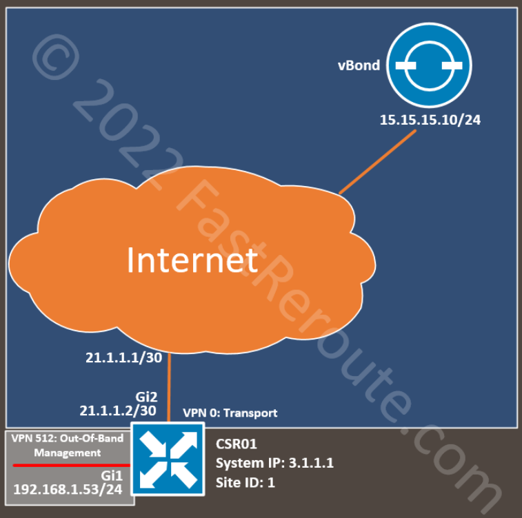
The procedure described in this article can be used as part of the bootstrap process of Cisco IOS-XE devices. We start with a CSR1000V SD-WAN edge router in CLI mode, registered with vManage.
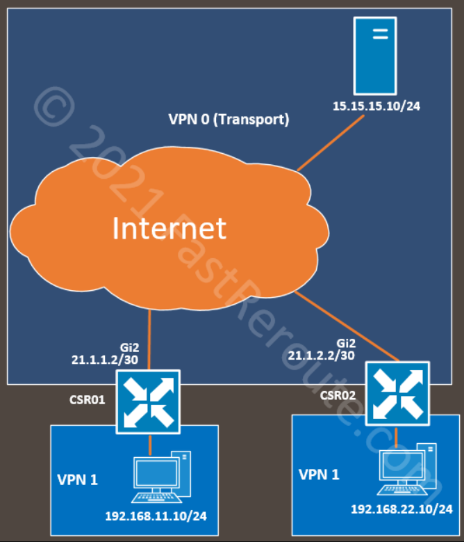
The topology has a single router connected to the Internet via an Ethernet interface. We configured the IP address on this interface and the default static route statically.
The configuration includes an out-of-band management interface, so we are not limited to console connectivity for troubleshooting and can use SSH over the Ethernet interface. This part of the configuration is optional, and you can skip the templates for out-of-band VPN 512.
Figure 1. SD-WAN templates sample topology
See the router’s basic CLI configuration in the listing below. We will substitute it with generated configuration from the feature and device templates while ensuring that the device is still able to connect to vManage.
We don’t use the service-side (LAN) configuration in this example. Additional templates can enable other settings after the device is switched to template-based management.
Base CLI Configuration
The basic configuration of the SD-WAN edge device includes the following details:
System parameters (lines 3-10)
Transport and tunnel interface configuration (lines 25-33, 41-45)
Transport VPN routing (line 35)
Out-Of-Band Management VPN and Interface (optional, lines 12-23)
config-transaction
!
system
 system-ip             3.1.1.1
 site-id               1
 admin-tech-on-failure
 organization-name     SD-WAN-TESTLAB
 vbond 100.1.1.51
!
hostname CSR01
!
vrf definition Mgmt-intf
 rd 1:512
 !
 address-family ipv4
  route-target export 1:512
  route-target import 1:512
 exit-address-family
exit
!
interface GigabitEthernet1
 vrf forwarding Mgmt-intf
 ip address 192.168.1.53 255.255.255.0
!
interface GigabitEthernet2
 no shutdown
 ip address 21.1.1.2 255.255.255.252
!
interface Tunnel0
 no shutdown
 ip unnumbered GigabitEthernet2
 tunnel source GigabitEthernet2
 tunnel mode sdwan
!
ip route 0.0.0.0 0.0.0.0 21.1.1.1
!
line vty 0 4
 transport input ssh
!
sdwan
 interface GigabitEthernet2
  tunnel-interface
   encapsulation ipsec
   color default
  exit
 exit
!
commit
Feature templates
In this article, we will create all feature templates from scratch.
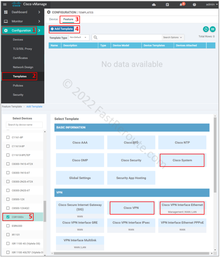
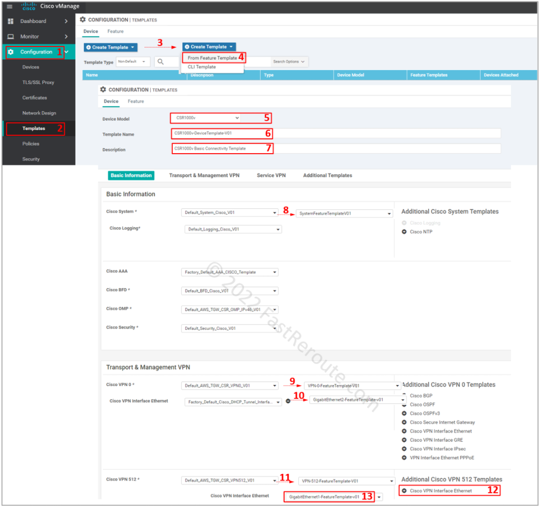
To add a feature template refer to the screenshot below.
Start by selecting Configuration > Templates in the side menu. Then click on the Feature tab and the “Add Template” button. Select CSR1000v as the device type. I highlighted the templates used in this article – System, VPN, and Ethernet.
Figure 2. Add new feature template
Step 1. System template configuration
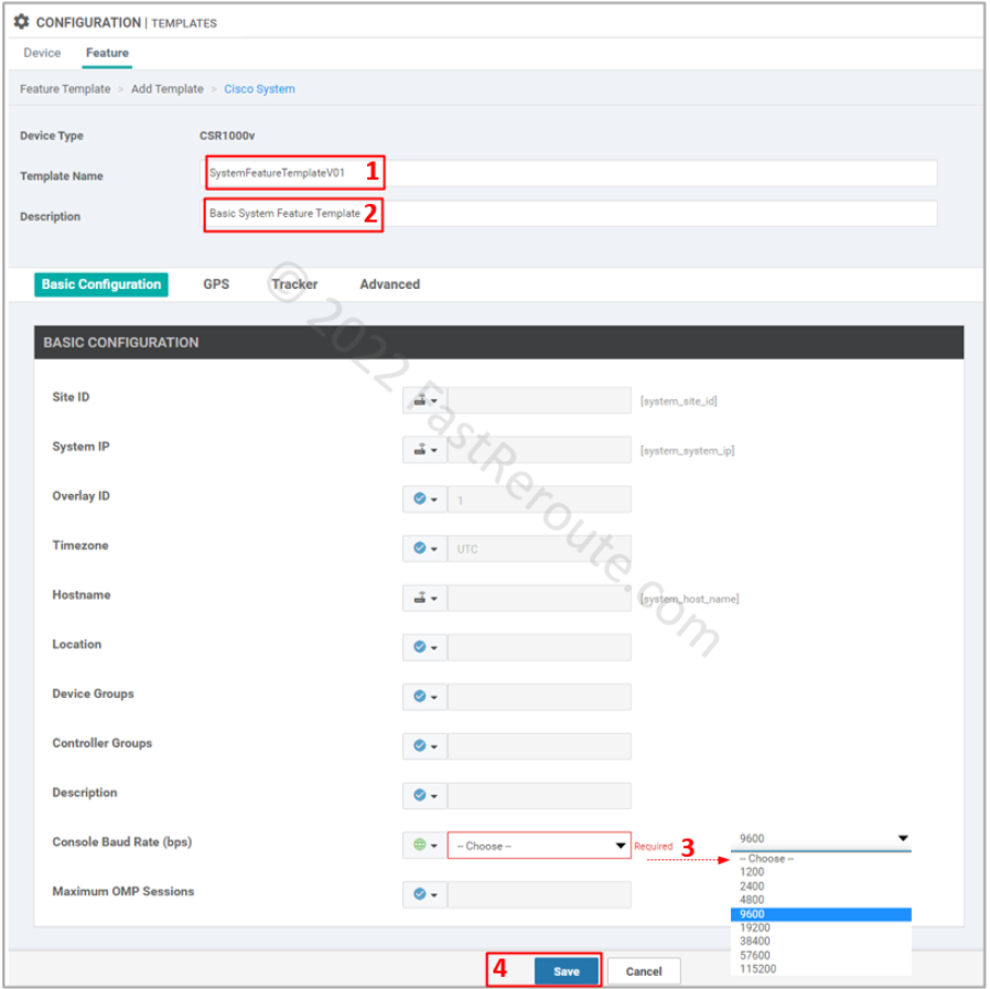
This template defines System IP, Site ID, and Hostname details. We want to generate the following configuration with the template:
To add a System template select the “Cisco System” button in the “Add Template” window shown in Figure 2. Set the name and description of the template.
Default options have variables defined for the parameters we want to define. The only mandatory setting is the Console Baud Rate, and figure 3 shows the required details.
Figure 3. System template configuration
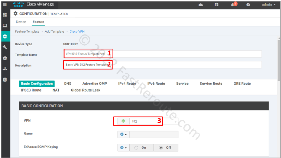
Step 2. Transport VPN
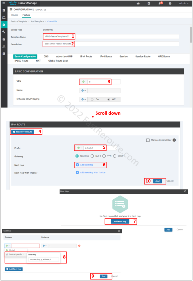
This template defines transport VPN, a global routing context (VRF 0) in Cisco IOS-XE. With this template, we aim to generate the static default route from the complete configuration:
ip route 0.0.0.0 0.0.0.0 21.1.1.1
To add it click on the “Cisco VPN” button on the add feature template page, shown in Figure 2. Add name and description of the template.
Figure 4. Transport VPN template configuration
Set VPN value of 0, which is reserved ID for transport VPN.
For our configuration, we need only specify a default route. To be able to re-use template, use a device variable for the next hop (vpn_next_hop_ip_address_0). This variable can be either the IP address of the next-hop or interface name for point-to-point connections.
Don’t forget to press Add button (#10), as the configuration window will not warn you that the route is not added, which will cause the device to lose connectivity to vManage. Not saving sub-configuration sections is a common issue, which can happen across many vManage configuration pages, as the Web user interface doesn’t force a user to save or discard when adding sub-elements.
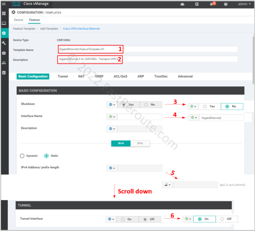
Step 3. Transport interface
This template generates the configuration shown below:
interface GigabitEthernet2
 no shutdown
 ip address 21.1.1.2 255.255.255.252
!
interface Tunnel0
 no shutdown
 ip unnumbered GigabitEthernet2
 tunnel source GigabitEthernet2
 tunnel mode sdwan
!
sdwan
 interface GigabitEthernet2
  tunnel-interface
   encapsulation ipsec
   color default
  exit
 exit
Use procedure from the first section to get to the Feature template selection (Figure 2) and then select “Cisco VPN Interface Ethernet” as the type.
Specify the template name and description. Change the following values:
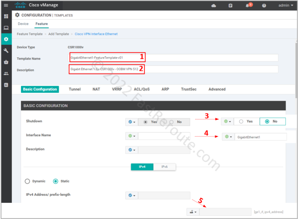
This configuration is similar to the previous two steps. The management VPN uses a reserved ID of 512. SD-WAN overlay doesn’t transport it over, which is why it is called out-of-band. You can only access it locally or expand it using a dedicated network.
In this example, we don’t set up any static routes in VPN 512, as we plan to connect to the device locally via port GigabitEthernet1. In your network, you can set up static routes without any risk to the transport or other VPNs, as each VPN is a VRF, which has its isolated routing table.
The interface configuration differs from the transport interface by not having the tunnel option enabled.
Figure 7. Management interface in VPN 512
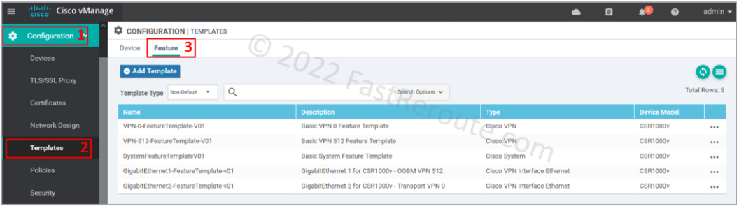
Step 5. Configure device template
We have created five feature templates, as shown in Figure 8.
Figure 8. Feature templates list
Let’s create a device template using the steps shown in Figure 9. Select device type, then provide a name and description for the template. Change the following templates:
Cisco System
Cisco VPN 0
Cisco VPN Interface Ethernet
Cisco VPN 512
Cisco VPN Interface Ethernet (add it first)
Figure 9. Create a device template
Cisco AAA template defines user authentication for out-of-band management access. The pre-configured AAA template defines default credentials – user/password combination of admin/admin. Use them to SSH to the device via VPN 512.
You should change it in the production network as a security precaution by defining a custom Cisco AAA template. Save the device template.
Step 6. Apply device template
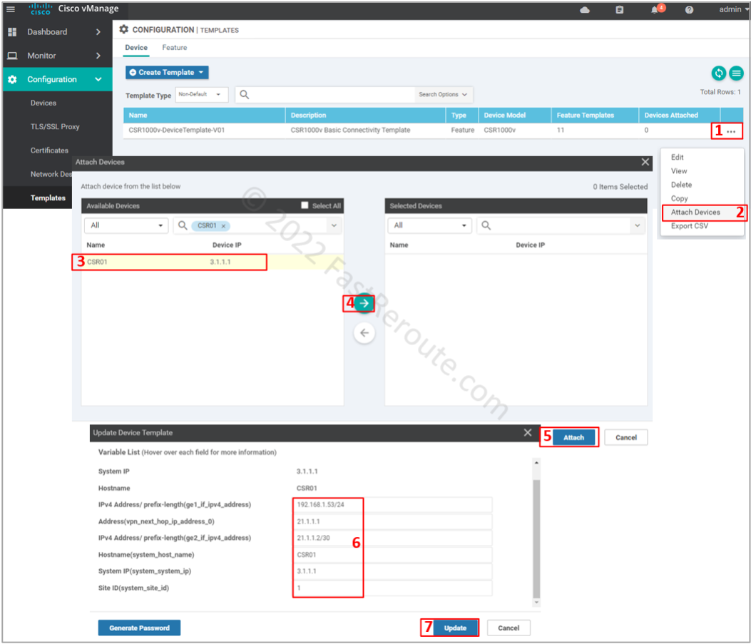
Now it’s time to apply the template to the device. Open the template configuration page select the device template created in the previous step. Click on the three dots column and then on Attach Devices.
Select CSR01, click on the right-pointing arrow, and then the Attach button.
Fill in values for the variables, which came from the templates defined earlier, and press Update.
List of variables and their values:
ge1_if_ipv4_address – 192.168.1.53/24
vpn_next_hop_ip_address_0 – 21.1.1.1
ge2_if_ipv4_address – 21.1.1.2/30
system_host_name – CSR01
system_system_ip – 3.1.1.1
system_site_id – 1
Figure 10. Apply the device template
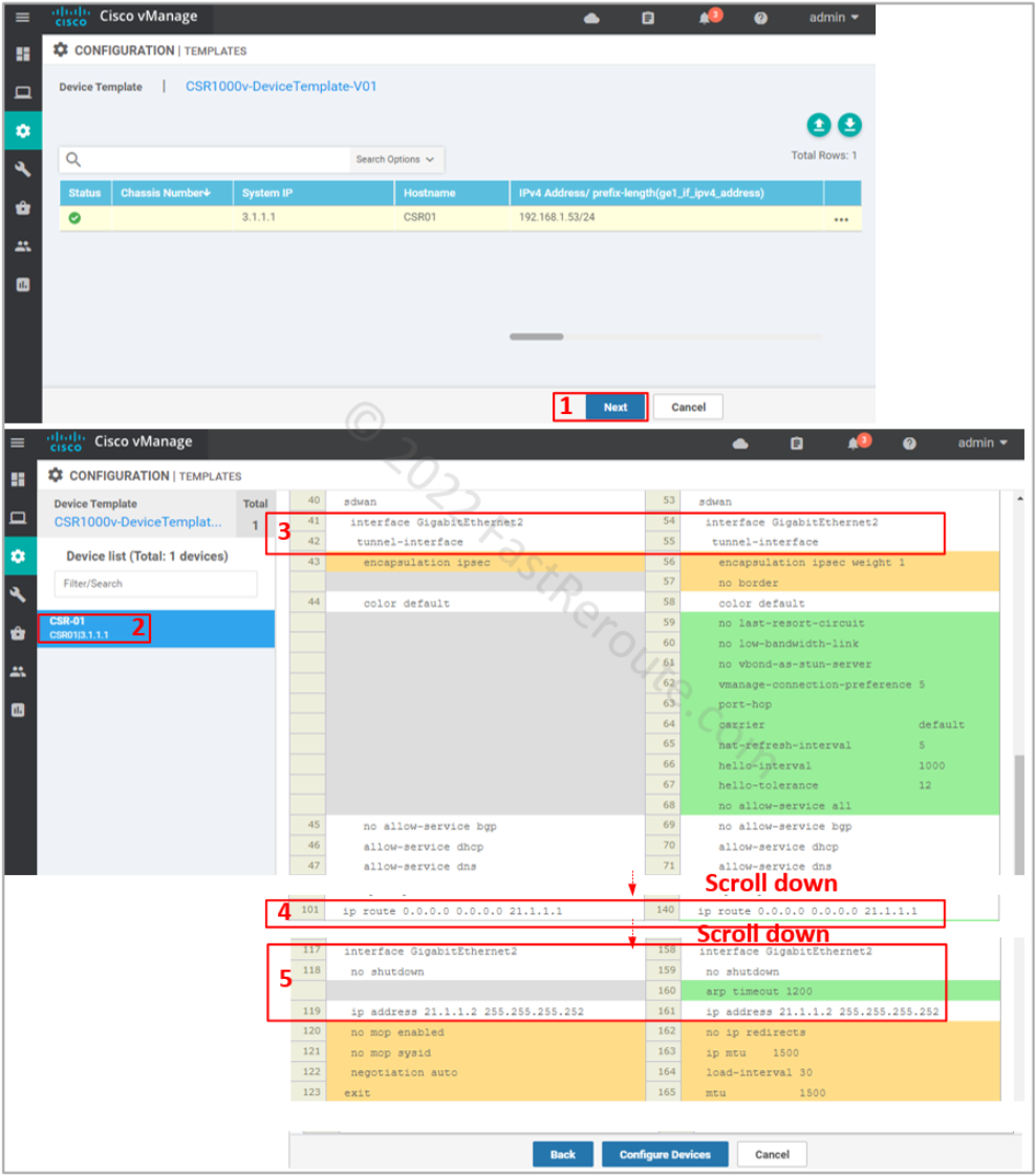
The final step is to check the configuration changes in CLI, as shown in Figure 11. Check the transport interface and VPN 0 static route.
In this blog post, we want to show how to enable a zone-based firewall on the Cisco SD-WAN platform. The example continues on the topology in the Direct Internet Access article. We introduced an additional site to demonstrate that the configuration applied doesn’t affect inter-site traffic.
The diagram below shows the topology with a PC behind CSR1. It can access the Internet without any restrictions after enabling Direct Internet Access. If we want to restrict what is reachable from the service side, two options are available – access lists attached to the internal interface and zone-based firewall functionality. As on the traditional, non-SD-WAN router, access-lists are used in scenarios when no stateful inspection is required, for example, when you want to drop RFC 1918 traffic coming from your guest WIFI segment. Cisco zone-based firewall adds the ability to identify the application and stateful inspection, which allows return traffic if it’s part of the permitted session.
Figure 1. Sample Topology
Initial setup for DIA blocking all outbound traffic
The first section will create and associate a security policy that will block all traffic from the internal network to the Internet.
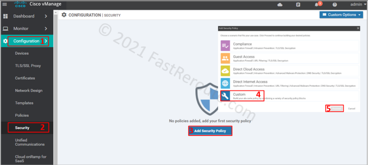
To apply the firewall rules, use a localized security policy. Navigate to Configuration > Policy. Click on Add Security Policy. Choose a custom policy from the list below, as this option shows all possible configuration elements.
Figure 2. Create a Security Policy
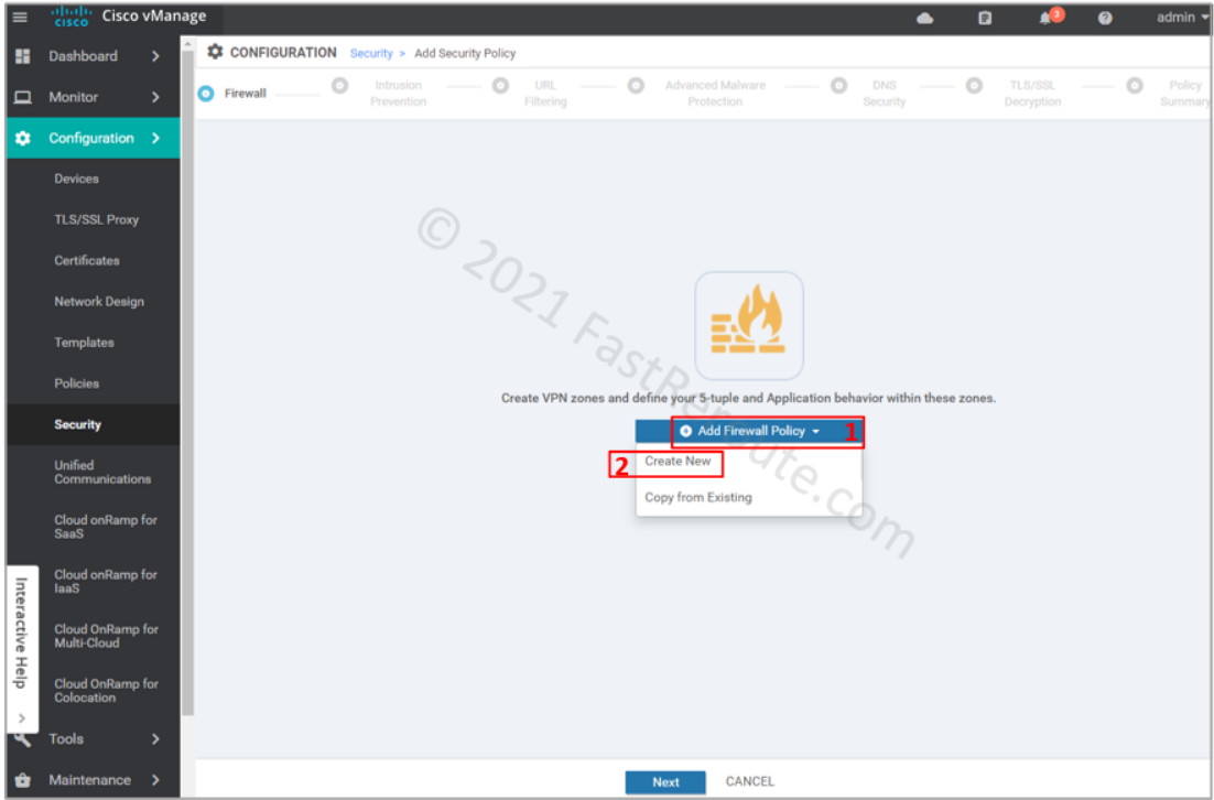
The first screen in the wizard is firewall configuration. Click on Add Firewall Policy, and then on Create New.
Figure 3. Add New Firewall Policy
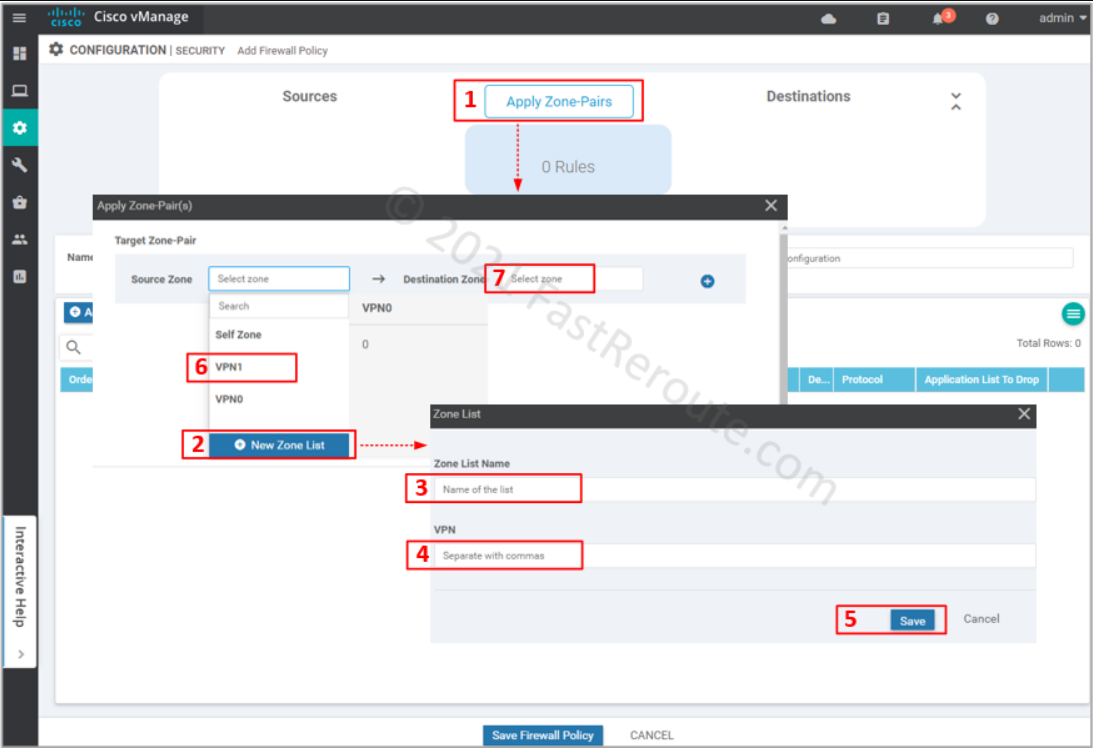
Define source and destination zone pairs by clicking on Apply Zone-Pairs button. Select source and destination zones. You can create zones within the wizard by specifying which VPNs will be part of them.
Figure 4. Define Security Zones
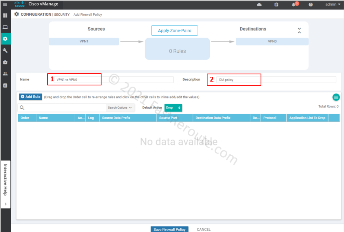
Provide Name and Description for the firewall policy. We can add rules as required; however, we want to drop all the traffic first. The default action, which is applied when no rules match the packet, is Drop (you can change this behavior by selecting Pass in the dropdown menu).
Figure 5. Name and Description of Security Policy
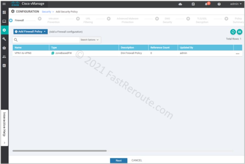
Review created firewall policy and press Next.
Figure 6. Firewall Policy Review
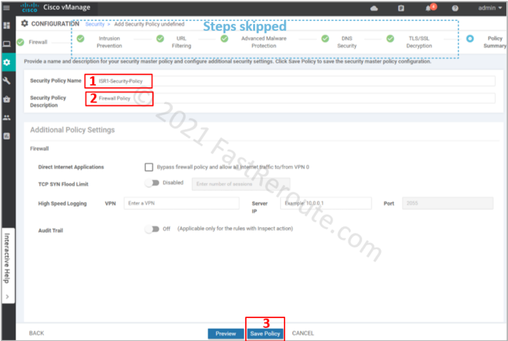
We’ve clicked through all remaining pages of the wizard without adding any configuration. On the “Policy summary” page, provide Security Policy Name and its description.
Figure 7. Security Policy Review
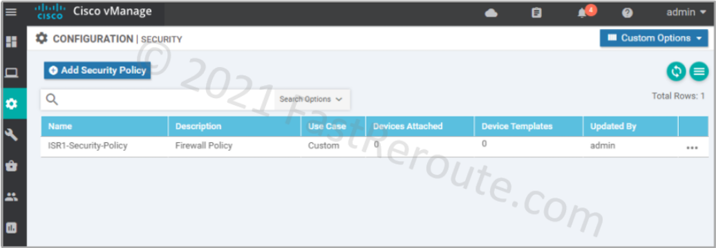
After clicking on the Save Policy button, we can see the policy we’ve just created in the list.
Figure 8. List of Security Policies
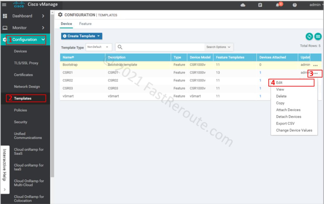
Now it’s time to apply the policy to the device. The device template applies the policy to the device.
Figure 9. List of Device Templates
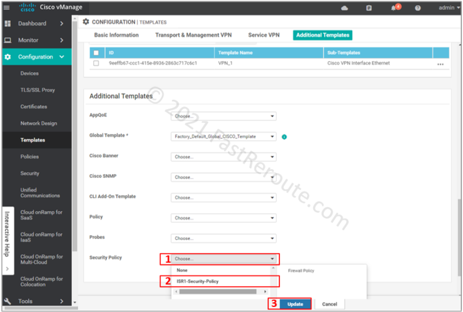
Choose ISR1-Security-Policy in the Security Policy dropdown. And press the Update button to push the configuration to the device.
Figure 10. Apply Security Policy to Template
The listing below shows the config lines are sent to the device based on the configuration we’ve made so far (you can check this via configuration difference preview before the configuration push). As we haven’t specified any specific rules, the policy uses only the class-default class with drop action. The ‘inspect’ firewall policy is defined and applied within the zone-pair configuration block.
parameter-map type inspect-global
 alert on
 log dropped-packets
 multi-tenancy
 vpn zone security

policy-map type inspect VPN1-to-VPN0
 class class-default
  drop

zone security VPN0
 vpn 0
zone security VPN1
 vpn 1
zone-pair security ZP_VPN1_VPN0_VPN1-to-VPN0 source VPN1 destination VPN0
 service-policy type inspect VPN1-to-VPN0
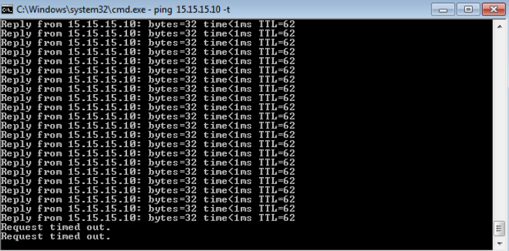
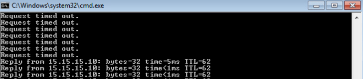
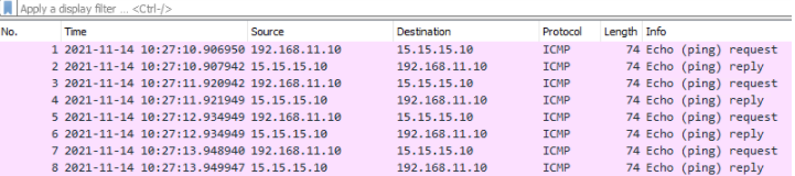
The test shows that the ICMP traffic is blocked as soon as the policy is applied.
Figure 11. Traffic to the Internet is now blocked
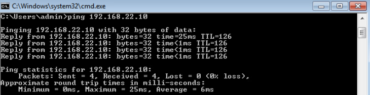
To demonstrate that our policy didn’t affect traffic within VPN 1, let’s ping the PC behind CSR02 at another site.
Figure 12. Site-to-site traffic is not affected
Adjust policy to allow ICMP traffic
This section will allow ICMP traffic to the Internet by modifying the policy.
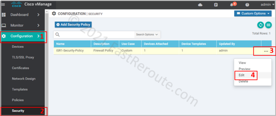
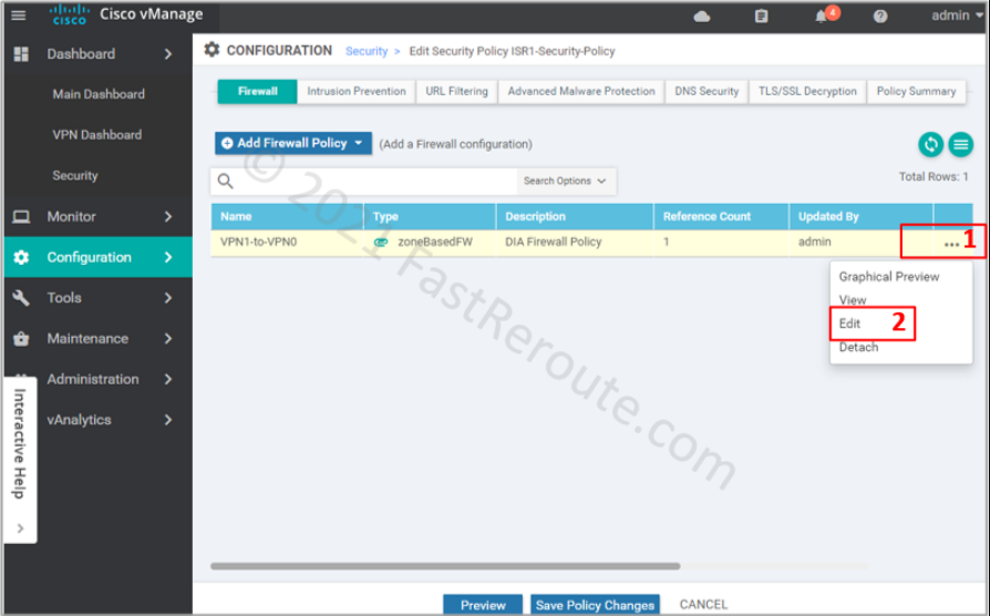
Return to the policy list via Configuration > Security. Choose the policy that we’ve created earlier and press Edit.
Figure 13. Edit existing security policy
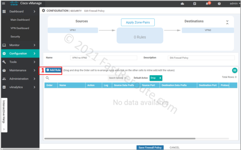
Click on the firewall section, choose the “VPN1-to-VPN0” firewall rule and press Edit.
Figure 14. Edit existing firewall policy
Add the new rule by clicking on the “Add Rule” button.
Figure 15. Add a rule to the firewall policy
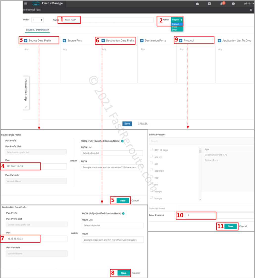
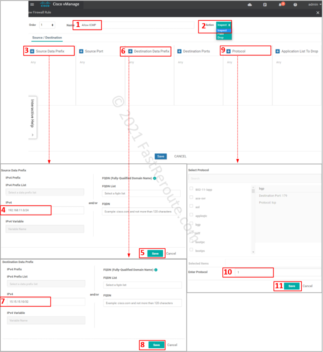
Specify ACL entry name and choose action to apply. Drop is self-descriptive. Inspect creates a stateful record of the session and automatically allows return traffic. Pass action – will not allow return traffic; for this action to work, you will be required to create another zone-pair for reverse direction and explicitly allow return traffic.
Define matching traffic and action. Protocol number 1 matches ICMP. Select one of the pre-defined protocols for TCP and UDP traffic. If unavailable or non-standard port numbers need to be specified, use ‘tcp’ or ‘udp’ as a protocol along with the “Destination Ports” condition.
Figure 16. Define the access-list entry
Review the rule, save it, and its parent firewall policy.
Figure 17. Firewall rule and policy summary
vManage sends the following commands to the device.
The first three commands are object groups that identify the source, destination, and protocol.
Then access list is defined using the object groups. The class map that follows uses the ACL as a “match” condition.
Finally, policy-map now has a custom class-map statement placed above the default. The action for this traffic is ‘inspect,’ so return packets are automatically allowed.
object-group network VPN1-to-VPN0-seq-Allow_ICMP-network-dstn-og_
 host 15.15.15.10
object-group network VPN1-to-VPN0-seq-Allow_ICMP-network-src-og_
 192.168.11.0 255.255.255.0
object-group service VPN1-to-VPN0-seq-Allow_ICMP-service-og_
 icmp

ip access-list extended VPN1-to-VPN0-seq-Allow_ICMP-acl_
 permit object-group VPN1-to-VPN0-seq-Allow_ICMP-service-og_ object-group VPN1-to-VPN0-seq-Allow_ICMP-network-src-og_ object-group VPN1-to-VPN0-seq-Allow_ICMP-network-dstn-og_

class-map type inspect match-all VPN1-to-VPN0-seq-1-cm_
 match access-group name VPN1-to-VPN0-seq-Allow_ICMP-acl_

policy-map type inspect VPN1-to-VPN0
 class type inspect VPN1-to-VPN0-seq-1-cm_
  inspect
 class class-default
  drop
Figure 18. ICMP traffic to the Internet is now allowed
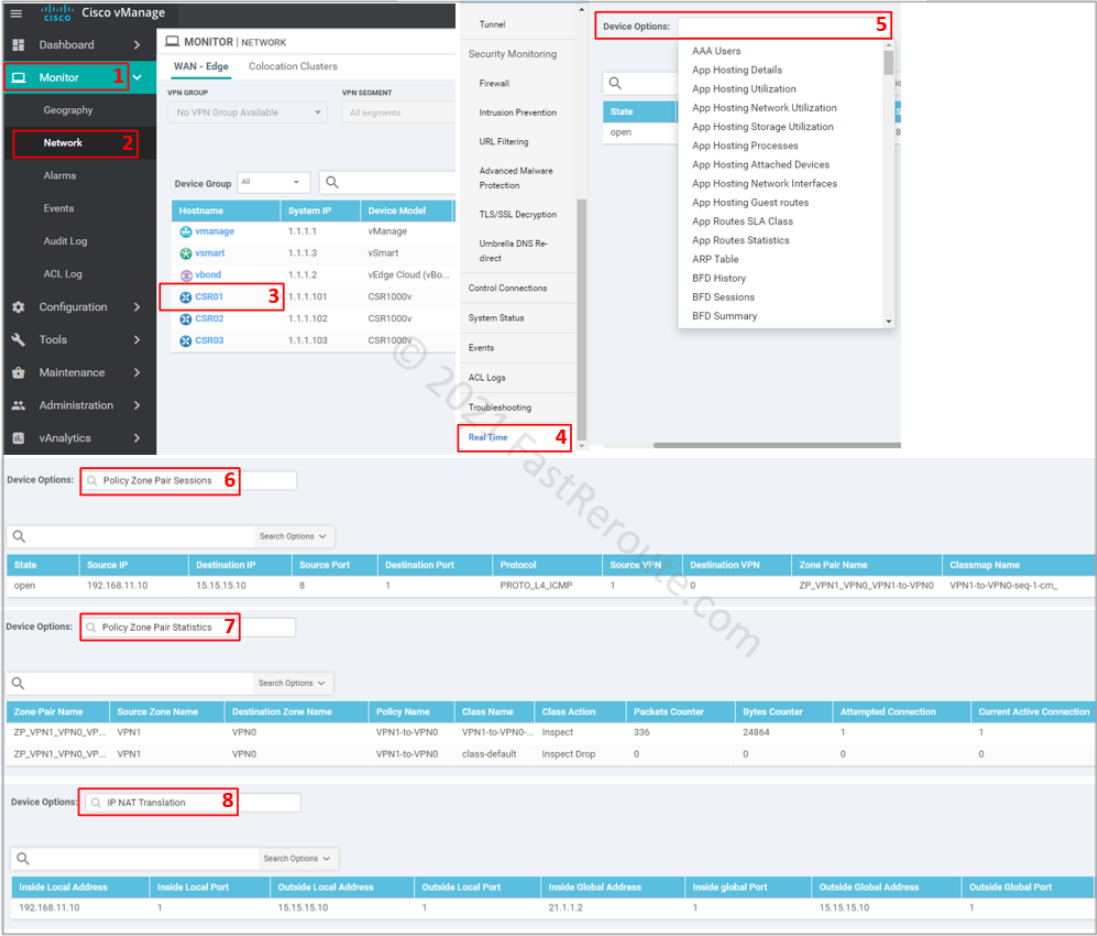
To monitor or troubleshoot firewall sessions, use the Real-Time menu in the device monitoring, as shown in the screenshot below. The following options provide relevant real-time information:
Policy Zone Pair Sessions – displays list of sessions and which zone pair and class map is matched for each session
Policy Zone Pair Statistics – shows statistics of packets and bytes matching per class-map
IP NAT Translation – displays NAT translations, which can be useful in DIA troubleshooting scenarios
Figure 19. Use vManage Web interface to view firewall sessions
To view active sessions using CLI as they are passing, use show policy-firewall sessions command:
CSR01#show policy-firewall sessions platform ?
  all                     detailed information
  destination-port        Destination Port Number
  detail                  detail on or off
  icmp                    Protocol Type ICMP
  imprecise               imprecise information
  session                 session information
  source-port             Source Port
  source-vrf              Source Vrf ID
  standby                 standby information
  tcp                     Protocol Type TCP
  udp                     Protocol Type UDP
  v4-destination-address  IPv4 Desination Address
  v4-source-address       IPv4 Source Address
  v6-destination-address  IPv6 Desination Address
  v6-source-address       IPv6 Source Address
  |                       Output modifiers
  <cr>                    <cr>
It is possible to filter the output using one of the keywords above. We will display all sessions with 'all' keyword.
CSR01#show policy-firewall sessions platform all
--show platform hardware qfp active feature firewall datapath scb any any any any any all any --
[s=session  i=imprecise channel c=control channel  d=data channel A/D=appfw action allow/deny]
Session ID:0x00000001 192.168.11.10 8 15.15.15.10 1 proto 1 (1:1:1:1) (0x3:icmp)        [sc]
To display detailed information on the session, which includes ingress and egress interfaces, translated addresses, and other information use detail keyword.
Packet capture provides a way of getting a copy of the packets traversing a router. This can be useful for troubleshooting purposes when you want to see if the packets are being received or sent by the router via the expected interface.
There are 2 ways to perform the packet capture – one is using the vManage user interface, and another one is using CLI directly on the router. In this article, we will explain how to use both of them.
Using vManage
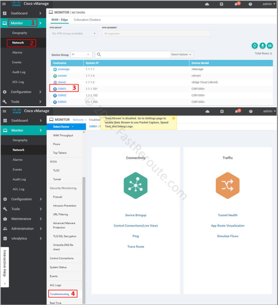
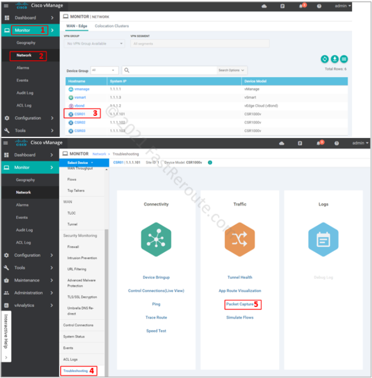
Packet capture is reachable via the Device Troubleshooting page – Monitor > Network > Device name > Troubleshooting. By default, there is no Packet Capture option under the Traffic section, as shown in Figure 1.
Figure 1. Packet Capture in vManage before Data Streaming is enabled
The pop-up alert displays: “Data Stream is disabled. Go to the Settings page to enable Data Stream to use Packet Capture, Speed Test, and Debug Logs”. To run packet captures via vManage we must enable Data Stream.
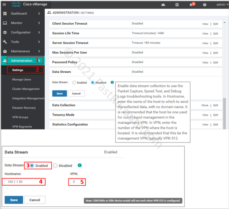
Navigate to Administration > Settings. Then expand the Data Stream option, as shown in the screenshot below. Click on the “Enabled” radio box, type in the hostname, which is the name or IP address of vManage and VPN that the edge router should use to reach the controller.
Figure 2. Enable Data Stream Configuration in vManage
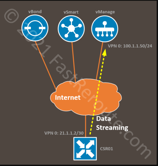
Note that for virtualized platforms, like the one we use for the lab, VPN 512 (out-of-band) cannot be used. To make this work, we are using the public IP of vManage, which is reachable via transport VPN 0. Our lab topology is shown in the figure below.
Figure 3. Data Streaming Topology
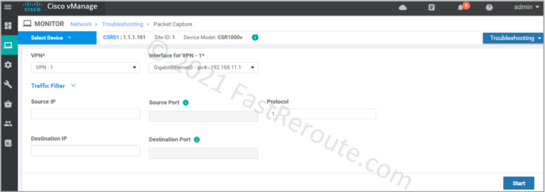
After enabling Data Streaming, the Packet Capture option is now visible in the Troubleshooting section. After clicking on this option, we can define packet capture parameters.
Figure 4. Packet Capture in vManage after Data Streaming is enabled
Packet capture screen requires VPN and Interface filter selection. You can optionally provide other filters, such as source and destination IPs and protocol information. Traffic is captured in both ingress and egress directions. Let’s change the filter to protocol 1 (ICMP) and start capture by pressing the Start button.
Figure 5. Packet Capture Parameters
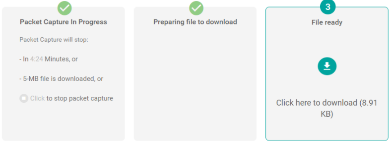
By default, the capture will run for 5 minutes. You can stop the timer at any time to download packets captured so far. The file in pcap format will be available for download shortly.
Figure 6. Packet Capture Progress
The content of the file can be viewed in Wireshark, as shown below.
Figure 7. Display Captured Packets in Wireshark
CSR01#show monitor capture

Status Information for Capture 71f87e76_847e_4770_8289_56b5242ac115
  Target Type:
 Interface: GigabitEthernet3, Direction: BOTH
   Status : Active
  Filter Details:
   IPv4
    Source IP:  any
    Destination IP:  any
   Protocol: 1
  Buffer Details:
   Buffer Type: LINEAR (default)
   Buffer Size (in MB): 5
  Limit Details:
   Number of Packets to capture: 0 (no limit)
   Packet Capture duration: 300
   Packet Size to capture: 0 (no limit)
   Maximum number of packets to capture per second: 1000
   Packet sampling rate: 0 (no sampling)
Using CLI on the router
If for some reason you can’t use vManage, you can use IOS-XE Embedded Packet Capture directly on the device (the previous process uses this feature on the backend). Use SSH to connect to the device either via client installed on your computer or via the tools menu in vManage.
The next configuration commands provide an example of running packet capture.
Embedded packet capture commands begin with monitor capture commands. They are available in exec mode, other operational commands, like “show” and “debug”.
CSR01#monitor capture ?
  WORD   Name of the Capture
  clear  Clear all Buffers
  start  Enable all capture points
  stop   Disable all capture points
Specify a name for the packet capture instance, in our example it is TEST_CAPTURE. The available command options are shown below.
CSR01#monitor capture TEST_CAPTURE ?
  WORD           Name of the Capture
  access-list    access-list to be attached
  buffer         Buffer options
  class-map      class name to attached
  clear          Clear Buffer
  control-plane  Control Plane
  export         Export Buffer
  interface      Interface
  limit          Limit Packets Captured
  match          Describe filters inline
  start          Enable Capture
  stop           Disable Capture
  stop_export    Disable Capture and Export Buffer
The next commands configure the same options we used in vManage:
GigabithEthernet3 as interface
ICMP packets only (IP protocol 1)
CSR01#monitor capture TEST_CAPTURE interface GigabitEthernet3 both
CSR01#monitor capture TEST_CAPTURE match ipv4 protocol 1 any any
Below are the available options for inline filters.
CSR01#monitor capture TEST_CAPTURE match ?
  any           all packets
  ipv4          IPv4 packets only
  ipv6          IPv6 packets only
  mac           MAC filter configuration
  pktlen-range  Packet length range to capture
CSR01#monitor capture TEST_CAPTURE match ipv4 ?
  A.B.C.D/nn  IPv4 source Prefix <network>/<length>, e.g., 192.168.0.0/16
  any         Any source prefix
  host        A single source host
  protocol    Protocols
CSR01#monitor capture TEST_CAPTURE match ipv4 protocol ?
  <0-255>  An IP protocol number
  tcp      Filter by TCP protocol
  udp      Filter by UDP protocol
CSR01#monitor capture TEST_CAPTURE match ipv4 protocol 1 ?
  A.B.C.D/nn  IPv4 source Prefix <network>/<length>, e.g., 192.168.0.0/16
  any         Any source prefix
  host        A single source host
CSR01#monitor capture TEST_CAPTURE match ipv4 protocol 1 any ?
  A.B.C.D/nn  IPv4 destination Prefix <network>/<length>, e.g., 192.168.0.0/16
  any         Any destination prefix
  host        A single destination host
To validate capture parameters run the command: show monitor capture TEST_CAPTURE. As shown in the listing below, by default, the capture will run till its buffer will reach 10MB.
CSR01#show monitor capture TEST_CAPTURE

Status Information for Capture TEST_CAPTURE
  Target Type:
 Interface: GigabitEthernet3, Direction: BOTH
   Status : Inactive
  Filter Details:
   IPv4
    Source IP:  any
    Destination IP:  any
   Protocol: 1
  Buffer Details:
   Buffer Type: LINEAR (default)
   Buffer Size (in MB): 10
  Limit Details:
   Number of Packets to capture: 0 (no limit)
   Packet Capture duration: 0 (no limit)
   Packet Size to capture: 0 (no limit)
   Maximum number of packets to capture per second: 1000
   Packet sampling rate: 0 (no sampling)
Now we can activate the defined capture.
CSR01#monitor capture TEST_CAPTURE start
After running some pings from a test PC connected to the service side via GigabitEthernet3, we can validate that packets are being captured. The brief format is shown below. Detailed and dump options display truncated and full packet content.
Let’s stop packet capture with the following command.
CSR01#monitor capture TEST_CAPTURE stop
To analyze packet capture buffer offline, use export it using the command shown below:
CSR01#monitor capture TEST_CAPTURE export ?
  bootflash:  Location of the file
  flash:      Location of the file
  ftp:        Location of the file
  http:       Location of the file
  https:      Location of the file
  pram:       Location of the file
  rcp:        Location of the file
  scp:        Location of the file
  sftp:       Location of the file
  tftp:       Location of the file

CSR01#monitor capture TEST_CAPTURE export bootflash:test_capture.pcap
Exported Successfully
SD-WAN deployments use the Internet as the transport to replace WAN networks traditionally designed to leverage centralized Internet access via the data center. Direct Internet Access (DIA) refers to the configuration when Internet-facing traffic breaks out directly from the branch router.
Is Network Address Translation (NAT) required for DIA to operate? Yes, NAT maintains a translation table, that tracks outbound sessions from the service side VPNs (LAN), so the return traffic can be sent back without having to leak service VPN routes into VPN 0.
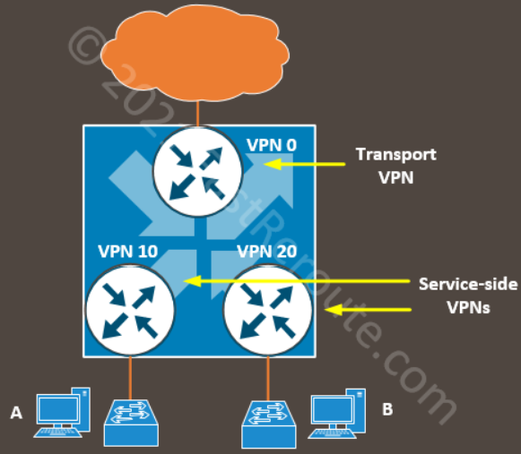
In the Cisco SD-WAN solution, transport-facing and user-facing interfaces belong to different VPNs or VRFs. VPN 0 contains transport (or underlay) network-facing interfaces, such as Internet and MPLS. Service-side VPNs contain user-facing interfaces.
The figure below shows logical VPN isolation within a router. In the routing table of VPN 0, there will be no entries for subnets where Host A and Host B are located. These subnets can even have the same IP addresses.
Figure 1. Transport and Service-Side VPNs and DIA
For DIA to work we need to allow traffic to flow between these virtual routers (or VPNs). To direct traffic from service-side VPNs we can use either static routes or a centralized data policy. NAT in transport VPN allows return traffic to be sent back.
Direct Internet Access on Cisco SD-WAN platforms is enabled in 2 steps. The first one is the NAT configuration on the transport interface. The second step directs traffic from service-side VPN using either a static route or centralized data policy.
Step 1: Enable NAT on the transport interface
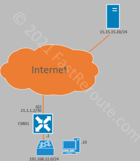
Let’s start with a very basic topology, shown in Figure 2.
Figure 2. Sample DIA Topology
Edge router has a device template assigned, which references a basic set of feature templates required to provide connectivity.
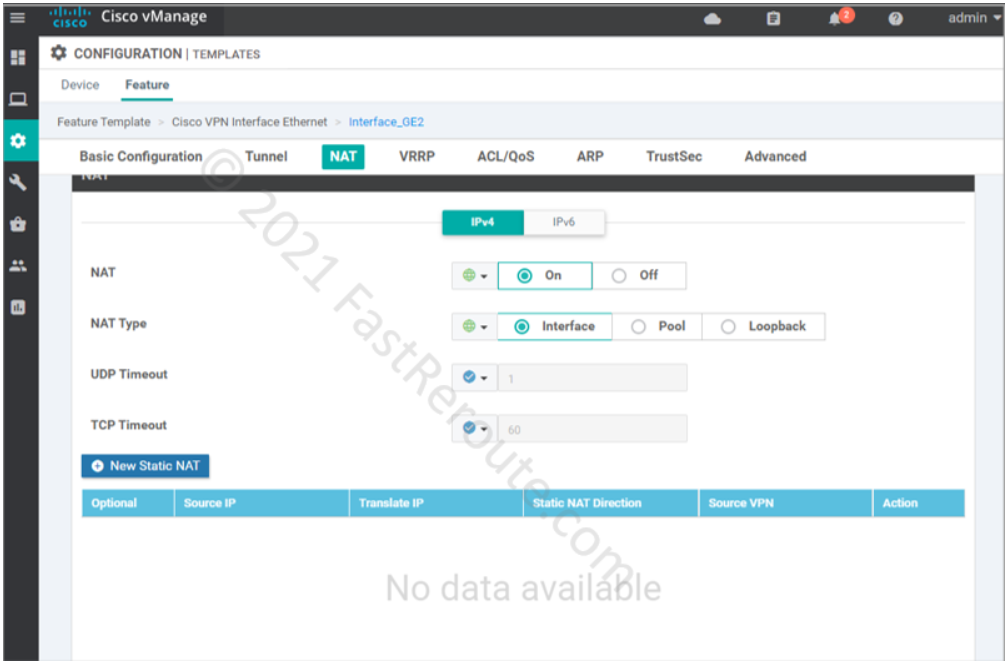
The first step of both static route and policy-based configuration is to enable NAT on an interface in the transport VPN – GigabitEthernet2. This is done by adjusting the interface template.
Figure 3. Enable NAT on transport interface
The following commands are pushed to the device.
ip nat inside source list nat-dia-vpn-hop-access-list interface GigabitEthernet2 overload
ip nat translation tcp-timeout 3600
ip nat translation udp-timeout 60

interface GigabitEthernet2
  ip nat outside
We couldn’t find a way to modify the nat-dia-vpn-hop-access-list used in ip nat insidecommand. This ACL is not visible in the running configuration or in the output of show ip access-lists. In IOS-XE this access list identifies traffic to be translated. In SD-WAN, however, to achieve this data policy needs to be configured.
Step 2: Direct traffic from service-side VPN
There are 2 ways to achieve this:
Static route in service VPN template
Centralized data policy
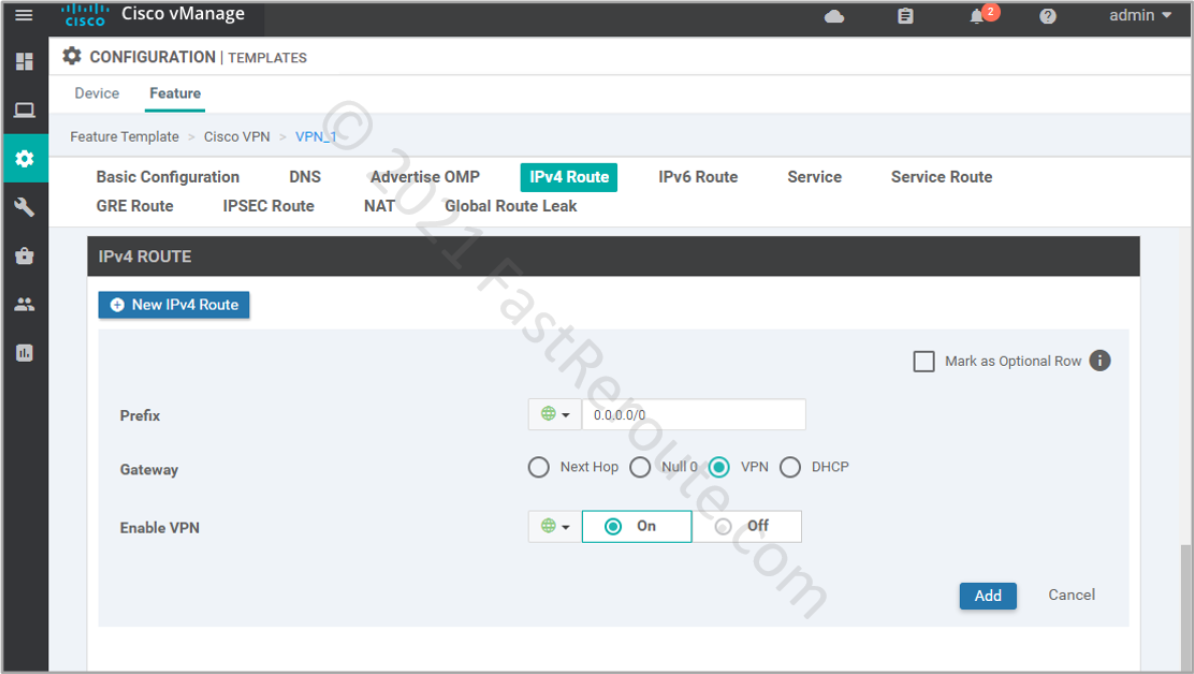
Step 2 (option 1): Static Route Configuration
Let’s configure a static default route under VPN 1 (Service VPN). Note that VPN is selected as a gateway option.
Figure 4. Configure a static default route
The static route command that is pushed to the device looks like this: ip nat route vrf 1 0.0.0.0 0.0.0.0 global
Note that the static route command has nat keyword. If we turn off NAT enabled in the previous step, the route will disappear. This essentially means that you have to do address translation for the configuration to work.
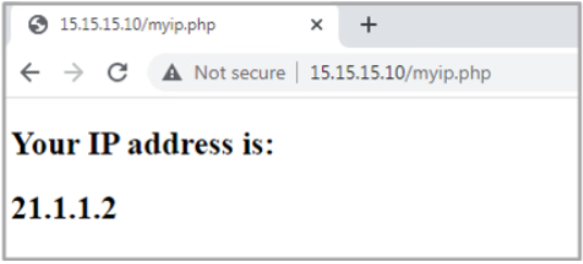
Let’s do the test from our test PC, confirming that the remote server sees the request as it’s coming from the router’s external IP address.
Figure 5. Test NAT configuration from Windows PC
To check the list of translations, we can run the following command on the router:
CSR01#show ip nat translations verbose
Pro  Inside global         Inside local          Outside local         Outside global
tcp  21.1.1.2:5062         192.168.11.10:49158   15.15.15.10:80        15.15.15.10:80
  create: 11/14/21 23:16:21, use: 11/14/21 23:16:27, timeout: 00:00:56
  RuleID : 1
  Flags: timing-out
  ALG Application Type: NA
  WLAN-Flags: unknown
  Mac-Address: 0000.0000.0000    Input-IDB:
  VRF: 1,  entry-id: 0xe9f7f840, use_count:1
  In_pkts: 7 In_bytes: 978, Out_pkts: 7 Out_bytes: 982
  Output-IDB: GigabitEthernet2

CSR01#show ip nat translation
Pro  Inside global         Inside local          Outside local         Outside global
tcp  21.1.1.2:5062         192.168.11.10:49158   15.15.15.10:80        15.15.15.10:80
Step 2 (Option 2): Centralized policy
We have removed the static route created in Step 2 (option 1), as the traffic will be directed by the centralized policy.
To implement DIA we will configure the traffic data section of the centralized policy that will match traffic coming from 192.168.11.0/24 (LAN segment) to 15.15.15.10/32 (the webserver).
Only one centralized policy can be activated globally at a time. The centralized policy contains multiple component policies. In this example, we will define a data policy, which then can be applied to a site list. In the following steps, we will create a new policy.
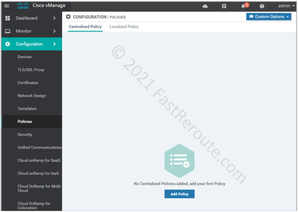
Create a centralized policy
Navigate to Configuration > Policies and click on Add Policy button.
Figure 6. Add Centralized Policy
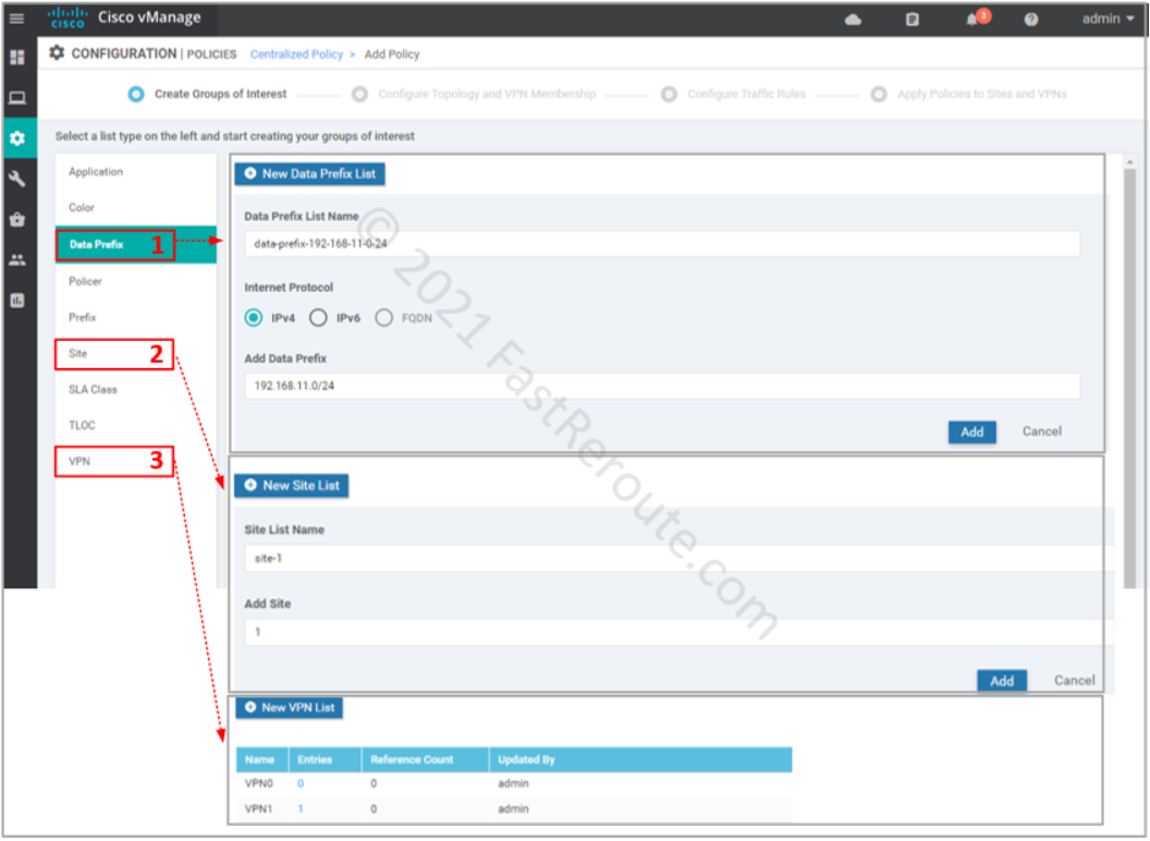
The first step of creating a policy is called “Create Groups of Interest”. These are variables that we can later use in the policy. For our example, we will define:
Data Prefix – for source prefix 192.168.11.0/24, and we will use 15.15.15.10/32 directly in our traffic matching configuration without variable definition
Site List – we want apply only to a single site with Site ID of 1; it is recommended not to have the same site in multiple site lists to ensure that only 1 policy of each type is applied to that site
VPN List – service VPN 1
Figure 7. Configure Groups of Interest (variables)
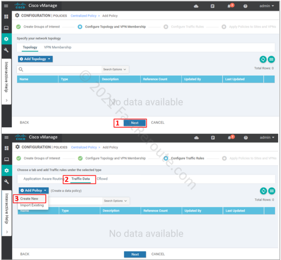
After defining all required variables and pressing the Next button, we are moved to the Topology and VPN Membership section of the wizard (see the top part of the screenshot below). We don’t need to configure anything for our data policy, so we just press Next.
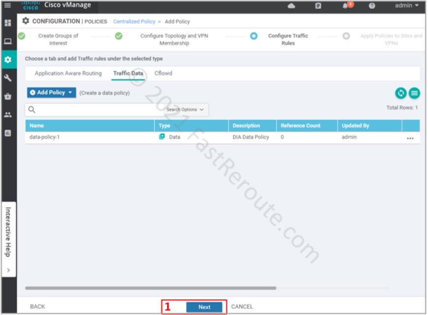
On the Configure Traffic Rules step of the wizard click on the “Traffic Data” section of the policy, click on Add Policy > Create New (refer to the bottom part of the next screenshot).
Figure 8. Configure Traffic Rules
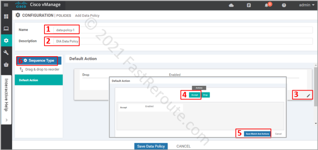
In a new data policy window enter the name and description of the policy. Adjust the default action to Accept to ensure that the packets that don’t match our criteria for DIA will not be dropped. Finally, press + button to add a rule that will be matching DIA traffic and apply NAT to it.
Figure 9. Create Data New Policy
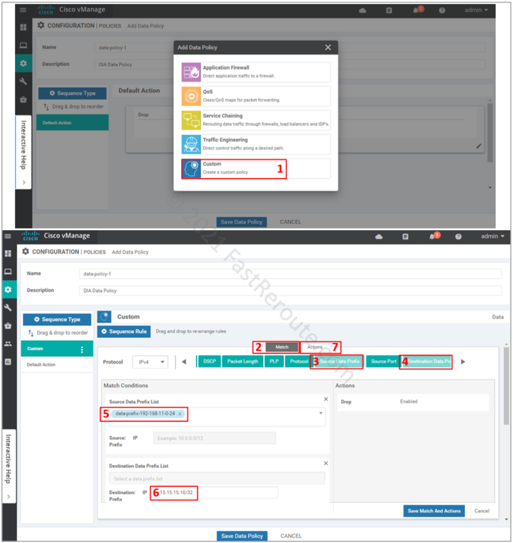
In the pop-up window select Custom policy. The other options are just a subset of the match and set conditions tailored for different scenarios, custom lists all of them.
Custom rule is added on top of the default action. If there are several rules, you can re-arrange them on the left panel. Ensure that the Match section is selected, add Source and Destination data prefixes to set the conditions for the rule.
Select the data prefix that we set up earlier in groups of interest as the source. Type-in destination as the actual address without the use of the variable. Both options lead to the same result, however, the use of variables allows you to use descriptive naming of the object plus adjusting the values outside of the policy configuration. Click on the Actions button.
Figure 10. Add a new custom rule to the policy and define match conditions
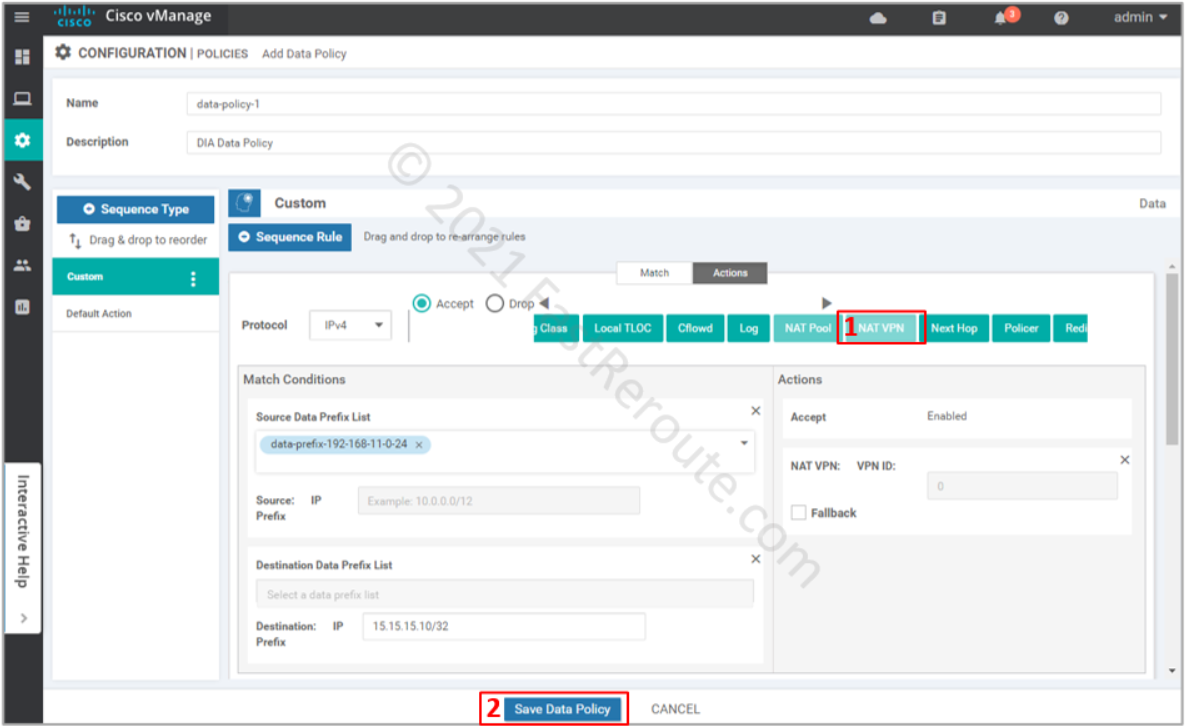
Select NAT VPN action, as shown in the following screenshot. The fallback option is useful when you want this traffic to follow the routing table when NAT cannot be used, for example, when the interface is down. Press the “Save data policy” button.
Figure 11. Set policy action to NAT VPN
The next screenshot list the data policy that we built in the previous step. Notice that the reference count is 0, as we haven’t yet applied it yet. Press Next.
Figure 12. Traffic data policies
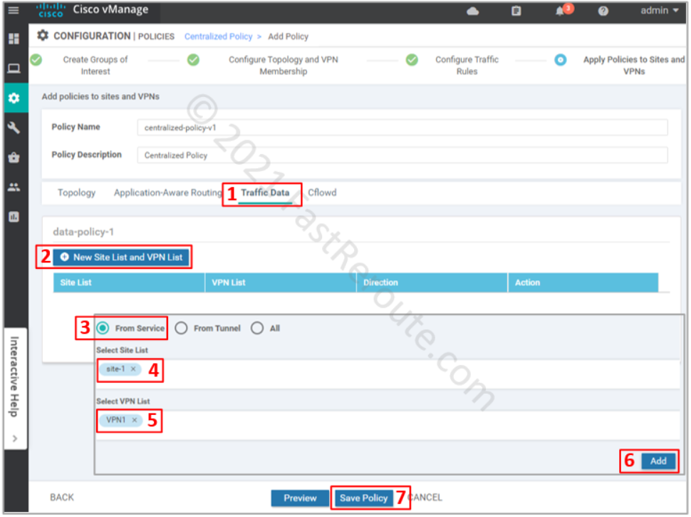
The final step is to apply the policy. Click on the Traffic Data section, and then under data-policy-1 press “New Site List and VPN List”. In the pop-up window select “From Service” direction, site-1 as the site list, and VPN1 as the VPN list. Press the Save Policy button.
Figure 13. Apply data policy
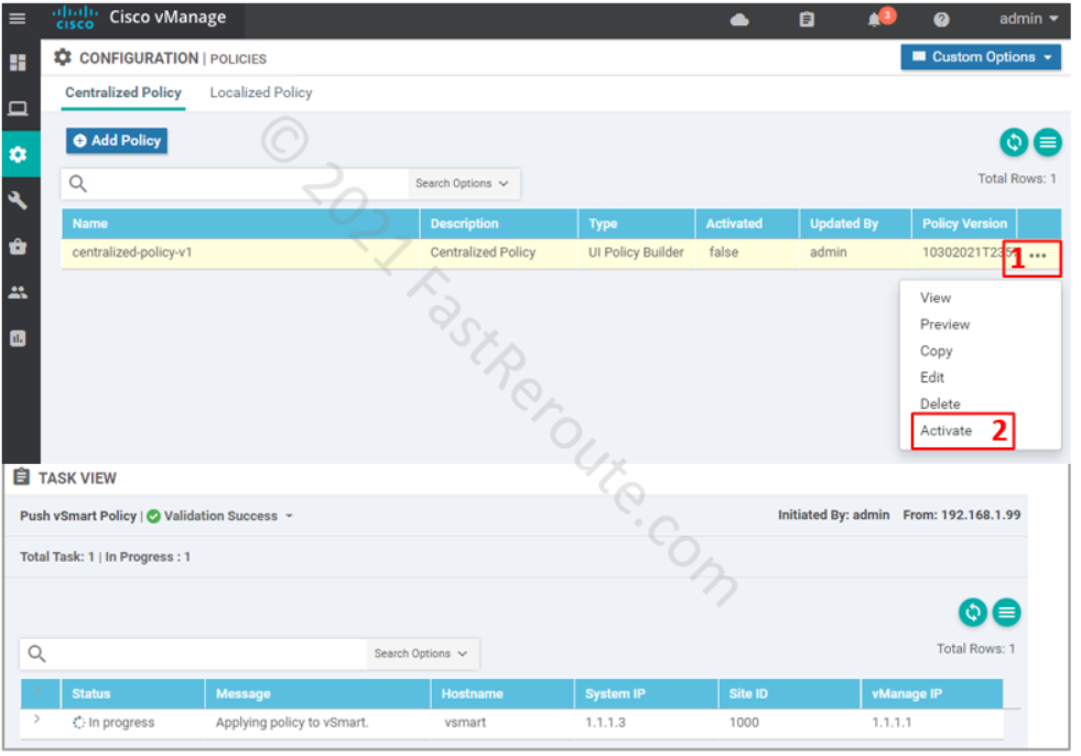
The final step is to activate the policy.
Figure 14. Activate centralized policy
At this stage vManage will push the policy to vSmart as part of its running-config:
vSmart will use OMP to distribute the policy to edge routers. In contrast to vSmart, edge routers will not display the policy in the running configuration. Use show sdwan policy from-vsmart command instead.
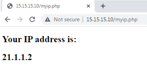
Let’s check from the client machine that NAT works:
CSR01#show ip nat translation
Pro  Inside global         Inside local          Outside local         Outside global
tcp  21.1.1.2:5064         192.168.11.10:62121   15.15.15.10:80        15.15.15.10:80
Cisco SD-WAN devices can be either in vManage or CLI mode.
In vManage mode, the configuration is performed on vManage and then pushed to the device. Local configuration changes are not allowed. In CLI mode, changes are performed locally on the device. vManage mode is the preferred and recommended option for most SD-WAN implementations. However, you can occasionally switch devices into CLI mode to perform specific tasks.
Administrators can connect to the device using SSH or serial console to use various show and debug commands in both modes.
We will focus on edge devices in this article. However, controllers can also be in one of these modes. Cisco-hosted controllers are initially provisioned in CLI mode and then converted to vManage mode by a network administrator. Some features require controllers to be switched to vManage mode.
vManage mode
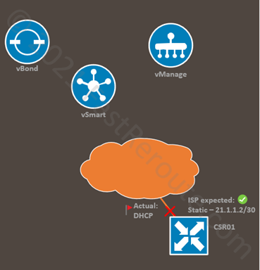
Consider a sample network shown in Figure 1. Our task is to prepare an edge router for a remote office. We’ve applied the required feature and device templates with dynamic IP assignment on the Internet-facing interface. After the router is shipped to the remote location and plugged in, it cannot establish connectivity to vManage. We discover that the ISP doesn’t have DHCP enabled, and a static IP configuration is required.
Figure 1. SD-WAN Edge Sample Scenario
Let’s assume that we can access the router via console cable attached to a laptop on-site.
Run the “show sdwan system status” command on the edge device to validate the device mode. In the sample output below, the CSR01 router is in vManage mode (vManaged: true).
CSR01#show sdwan system status
Viptela (tm) vEdge Operating System Software
Copyright (c) 2013-2021 by Viptela, Inc.
Controller Compatibility: 20.3
Version: 17.03.03.0.4762

<output omitted>

Personality:             vEdge
Model name:              CSR1000V
Services:                None
vManaged:                true
Commit pending:          false
Configuration template:  CSR01

<output omitted>
Firstly, we try to set a static IP address on the transport interface using CLI. We use the “config-t” command to enter the configuration mode. The “commit” command activates the configuration.
CSR01#config-t
CSR01(config)# interface GigabitEthernet 2
CSR01(config-if)# ip address 21.1.1.2 255.255.255.252
CSR01(config-if)# commit
The following warnings were generated:
  'system is-vmanaged': This device is being managed by the vManage. Any configuration changes to this device will be overwritten by the vManage after the control connection to the vManage comes back up.
Proceed? [yes,no] yes
Commit complete.

CSR01#show run interface GigabitEthernet 2
Building configuration...

<output omitted>

interface GigabitEthernet2
 description Transport Interface
 ip address 21.1.1.2 255.255.255.252
In our example, we didn’t have connectivity to vManage, so the changes were committed. However, as the warning message above advises vManage will overwrite modifications done on the device (see the example in the following listing) once the control connection is up.
CSR01#show run interface GigabitEthernet 2
Building configuration...

<output omitted>

interface GigabitEthernet2
 description Transport Interface
 ip address dhcp
Rollback to the original configuration (i.e. setting dynamic IP on the transport interface) causes connectivity to vManage fail, which introduces the connectivity problem we tried to solve in the first place. When we have connectivity to vManage, the CLI commands are just rejected, as shown in the listing below. vManage mode doesn’t permit changes on the edge device.
CSR01#config-t
CSR01(config)# interface GigabitEthernet2
CSR01(config-if)# ip address 21.1.1.2 255.255.255.252
CSR01(config-if)# commit
Aborted: 'system is-vmanaged': This device is being managed by the vManage. Configuration through the CLI is not allowed.
CLI Mode
There are several solutions to the problem described above. The first is to switch the device into CLI mode beforehand before sending it to the remote location. We can then adjust the configuration and set static IP address, and move the device back to vManage mode.
The second solution is using hidden support commands, which is not a supported way of configuring the device unless directed by Cisco TAC. However, it works and can be helpful in lab environments or as a quick fix to get the branch running (with full router reset later).
Let’s see how both options work with the examples below.
Switching device to CLI mode via vManage
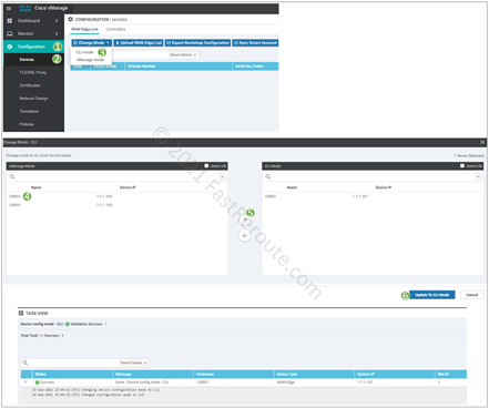
An administrator can switch the device to CLI mode (and back) via vManage. Navigate to Configuration > Devices. Click on the Change Mode drop-down menu and select CLI mode.
Figure 2. Switching device to CLI mode via vManage
In the dialog window, select and move to the right panel the router you want to switch into CLI mode and click on Upgrade to CLI Mode.
After the conversion, we can use “show sdwan system status” command to validate that the vManaged property is false.
CSR01#show sdwan system status
Viptela (tm) vEdge Operating System Software
Copyright (c) 2013-2021 by Viptela, Inc.
Controller Compatibility: 20.3
Version: 17.03.03.0.4762
Build: Not applicable

<output omitted>

Personality:             vEdge
Model name:              CSR1000V
Services:                None
vManaged:                false
Commit pending:          false
Configuration template:  None

<output omitted>
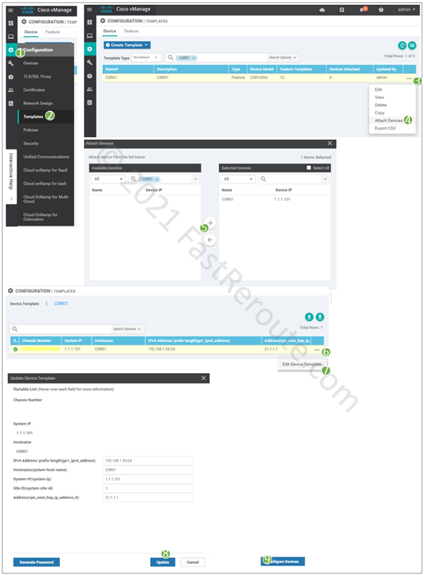
After the device comes back online, we can update templates to include static IP address configuration and switch it back to the vManage mode. To do this, we need to attach the device template to the vEdge router. If the device had a template attached before, the variable values would be populated automatically.
Figure 3. Switching device to vManage mode
Switching device to CLI mode using hidden commands
This procedure in this section uses hidden commands and should be used only as a last resort. Cisco TAC may not support it; use it at your own risk.
When the router hasn’t been switched to CLI mode beforehand and cannot establish a control connection to vManage, refer to the following example to switch to CLI mode.
After entering the configuration mode, let’s see available options under the system command:
CSR01#config-t
CSR01(config)# system ?
Possible completions:
  admin-tech-on-failure      Collect admin-tech before reboot due to daemon failure
  allow-same-site-tunnels    Allow tunnels to be formed between vEdges in the same site
  console-baud-rate          Console baud-rate
  control-session-pps        Control session policer rate, in packets per second
  controller-group-list      Controller group list
  debug
  description                System description
  device-groups              List of vManage groups to which the device belongs
  disable
  domain-id                  Domain ID
  environment
  fnf
  gps-location               GPS latitude and longitude of the device
  host-policer-pps           Rate at which to police packets bound to the control plane (in pps) per QOS level
  icmp-error-pps             Rate at which to police ICMP error messages either generated or received (in pps).
  idle-timeout               Idle CLI timeout, in minutes
  ignore
  location                   Location description of the device
  max-controllers            (DEPRECATED) Set the maximum number of controllers to which the device can connect - Deprecated in 15.4
  max-omp-sessions           Set the maximum number of OMP sessions the device can have
  mode-button
  mtu
  on-demand                  Set various configuration for On-demand tunnels
  organization-name          Organization name
  overlay-id                 Overlay ID
  port-hop                   Enable port hopping for all tlocs
  port-offset                Port offset (unique value; use only if multiple Viptela devices are behind the same NAT)
  site-id                    Site ID
  sp-organization-name       Service Provider Organization name
  system-ip                  System IP address
  system-tunnel-mtu          Control tunnel MTU
  tcp-optimization-enabled   Carve out a dedicated core to use for TCP optimization - applies after reboot
  timer                      Set various timer timeouts
  tls                        ssl-opt cert management config
  track-default-gateway      Enable/Disable default gateway tracking
  track-interface-tag        OMP Tag attached to routes based on interface tracking
  track-transport            Enable transport tracking
  upgrade-confirm            Configure software upgrade confirmation timeout
  vbond                      Configure remote vBond or local IPv4 vbond address
  <cr>
“unhide viptela_internal” command enables the display of “system” command hidden options. The example below shows these subcommands.
CSR01(config)# unhide viptela_internal
CSR01(config)# system ?
Possible completions:
  admin-tech-on-failure          Collect admin-tech before reboot due to daemon failure
  allow-same-site-tunnels        Allow tunnels to be formed between vEdges in the same site
  allow-sw-vedge                 (HIDDEN) Allow non-release software vedges to operate without certificates
  console-baud-rate              Console baud-rate
  control-session-pps            Control session policer rate, in packets per second
  controller-group-list          Controller group list
  daemon-reboot                  (HIDDEN) Reboot device if a non-restartable daemon fails
  daemon-restart                 (HIDDEN) Restart restartable daemons if they fail
  debug
  description                    System description
  device-groups                  List of vManage groups to which the device belongs
  disable
  dnsd-ttl                       config DNS reply TTL in secs
  domain-id                      Domain ID
  dpi-cache-expiry               (HIDDEN) Cache expiry time in minutes
  dpi-cache-size                 (HIDDEN) Cache size
  dpi-disable-track-tx           (HIDDEN) Enable/Disable DPI TRACK TX
  dpi-enable                     (HIDDEN) Enable/Disable DPI
  dpi-gc-time                    (HIDDEN) Garbage collect time in secs
  dpi-multicore                  (HIDDEN) Enable multi-core for dpi
  dpi-stat-time                  (HIDDEN) Stats collection time for dpi
  environment
  fnf
  fp-buffer-check                (HIDDEN) Enable fastpath buffer validity check
  fp-qos-interval                config fp qos interval
  fp-qos-weight-percent-factor   config fp qos weight percent factor
  gps-location                   GPS latitude and longitude of the device
  host-policer-pps               Rate at which to police packets bound to the control plane (in pps) per QOS level
  icmp-error-pps                 Rate at which to police ICMP error messages either generated or received (in pps).
  idle-timeout                   Idle CLI timeout, in minutes
  ignore
  increase-bp-count              (HIDDEN) Increase port backpressure threshold for all ports
  is-vmanaged                    Device is managed by the vmanage
  last-vmanage-transaction-id    Used by vManage to maintain integrity of transactions initiated by it towards device
  location                       Location description of the device
  max-controllers                (DEPRECATED) Set the maximum number of controllers to which the device can connect - Deprecated in 15.4
  max-omp-sessions               Set the maximum number of OMP sessions the device can have
  mode-button
  mtu
  on-demand                      Set various configuration for On-demand tunnels
  organization-name              Organization name
  overlay-id                     Overlay ID
  patch-confirm                  (HIDDEN) Configure software patch confirmation timeout
  port-bp-threshold              configure port backpressure threshold
  port-hop                       Enable port hopping for all tlocs
  port-offset                    Port offset (unique value; use only if multiple Viptela devices are behind the same NAT)
  pseudo-confirm-commit          Only valid for vmanage ..
  reboot-on-failure              (HIDDEN) Reboot device if any daemon fails
  simulated-color                Simulated device's color
  simulated-devices              Additional number of simulated devices
  simulated-wan-ip               Starting IP address for the simulated interface
  site-id                        Site ID
  sp-organization-name           Service Provider Organization name
  system-ip                      System IP address
  system-tunnel-mtu              Control tunnel MTU
  tcp-optimization-enabled       Carve out a dedicated core to use for TCP optimization - applies after reboot
  timer                          Set various timer timeouts
  tls                            ssl-opt cert management config
  track-default-gateway          Enable/Disable default gateway tracking
  track-interface-tag            OMP Tag attached to routes based on interface tracking
  track-transport                Enable transport tracking
  unpin-flows-with-reboot        (HIDDEN) Enable with reboot OR Disable flow pinning to FP cores
  upgrade-confirm                Configure software upgrade confirmation timeout
  vbond                          Configure remote vBond or local IPv4 vbond address
  ztp-status                     ZTP status
  <cr>
To switch the device to CLI mode, use is-vmanaged option.
CSR01(config)# interface GigabitEthernet 2
CSR01(config-if)# ip address 21.1.1.2 255.255.255.0
CSR01(config-if)# commit
Aborted: 'system is-vmanaged': This device is being managed by the vManage. Configuration through the CLI is not allowed.

CSR01(config-if)# exit
CSR01(config)# system is-vmanaged false
CSR01(config-system)# commit
Commit complete.
CSR01#show run int GigabitEthernet 2
Building configuration...

interface GigabitEthernet2
 description Transport Interface
 ip dhcp client default-router distance 1
 ip address 21.1.1.2 255.255.255.0
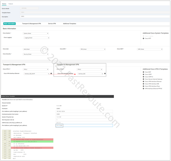
The device will connect to vManage. However, the controller will not overwrite the configuration. At this stage, vManage’s view of the router configuration will not reflect the actual state. We need to remediate this as soon as possible, either by switching the device to CLI mode or applying a configuration template that brings consistency. Let’s update the device template to use static interface configuration to get to the consistent state. In the screenshot below, we see the template adjustments. The bottom part of the figure contains the snippet of the command difference. As we saw in the previous command listing, the device already had a static IP address configured, but vManage is not aware of that change, so from its perspective, the device still has DHCP settings configured.
Figure 4. Apply Device Template to WAN Edge
Changing WAN Edge System IP
In the final section of this blog post, let’s see another example when switching to CLI mode can be helpful. When done via template change, the change of System IP can cause the configuration push to be stuck and not apply correctly.
As a workaround, you can switch the device into CLI mode, change System IP, and move it to template configuration back. Follow the steps below.
Step 1. To switch the device to CLI mode, refer to the procedure described in the first section and Figure 2.
Step 2. Using CLI apply the configuration change. In the example below, we change System IP from 1.1.1.101 to 1.1.1.11.
Step 3. Move device to vManaged mode by applying template and ensuring that the System IP variable matches the new value.
This blog post describes configuring a site-to-site IPsec VPN tunnel from a Cisco SD-WAN IOS-XE-based router to a non-SD-WAN device.
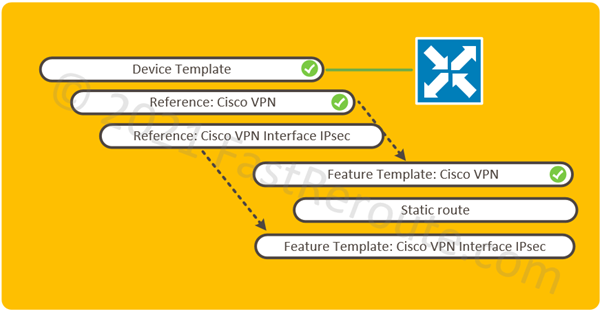
How to enable configure Cisco SD-WAN IPsec Tunnels to a non-SD-WAN device? In Cisco SD-WAN template-based deployment, IPsec tunnels are configured via the Cisco VPN Interface IPsec feature template. This template is then applied to the Transport VPN (0) or one of the Service VPNs.
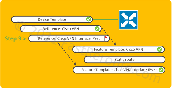
Cisco SD-WAN IPSec Tunnels Step-by-step
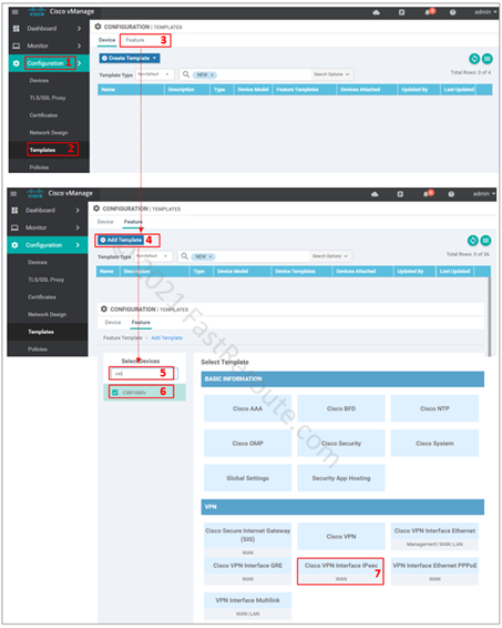
Figure 1. Configuration Map: Elements Diagram
The logical elements required to be configured shown in Figure 1. All pre-configured elements have check mark symbols next to them.
In our example, the edge device has a device template attached with basic configuration applied, such as system and transport interfaces, sufficient for the router to have control connections to the controllers.
The device template uses a service VPN, which is described by the Cisco VPN feature template. This type of template, despite its name, is not related to IPsec VPN settings. Cisco VPN feature template defines VRF settings and is a container for routing and participating interface information. In our example, the user-facing interface is assumed to be configured and associated with the VRF.
While it is possible to configure all child templates from within the device template, in our example, we will pre-configure child feature templates first and then select them in the device template.
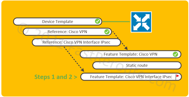
Create and Configure Cisco VPN Interface IPsec Feature Template
The first two steps deal with configuration of IPsec feature template.
Select model of devices that this feature template will be applied
Select Cisco VPN Interface IPsec
Figure 3. Create new feature template in vManage
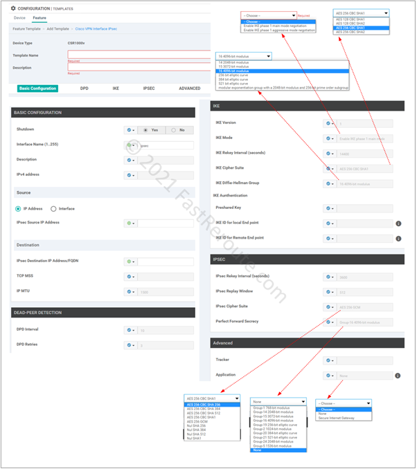
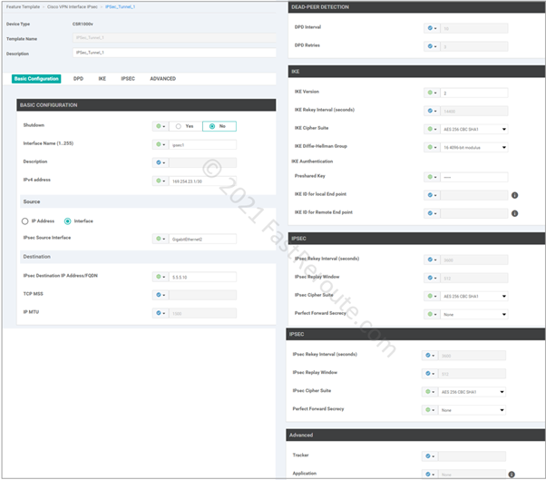
Step 2. Configure feature template
Customize IPSec tunnel parameters. There are 5 sections in IPsec template:
Basic configuration, such as name and IP address of the tunnel interface and its underlying source (local router) and destination (remote router)
Dead-peer detection settings
IKE or Phase 1 parameters
IPSEC or Phase 2 parameters
Advanced Settings
SD-WAN requires an IP-numbered interface (/30) and supports route-based tunnels known as VTI (Virtual Template Interface) in Cisco IOS documentation.
Instead of specifying interesting traffic using ACL known as policy-based tunnels, route-based tunnels use static or dynamic routing over a tunnel interface.
Figure 4. Configure feature template in vManage
As figure 4 shows, there are various options available for both IKE and IPSEC security parameters. These need to match between tunnel endpoints.
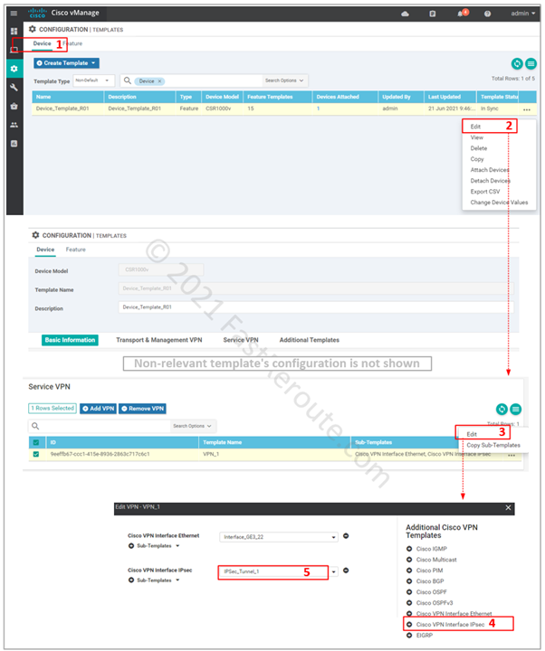
Adjust device template to use IPsec Feature Template
Step 3. Add feature template to the device template.
IPsec interface template can now be attached to the service VPNs. Figure 6 shows how to modify the existing device template.
Figure 6. Add IPsec template to service-side VPN.
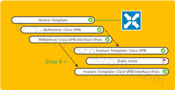
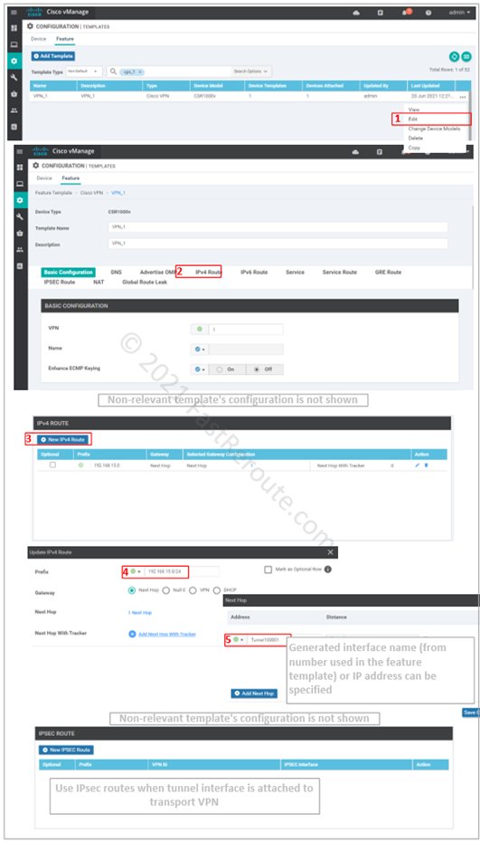
Routing Configuration
Figure 7. Configuration Map: Static Routes over IPsec interface
Step 4. Set-up routing over the tunnel. This can be static or dynamic-routing protocol-based. In the screenshot below, the static route configuration is shown.
Figure 8. Configure routing over IPsec tunnels
Step 5. Test the tunnel.
As the tunnels are VTI-based and have Layer 3 addresses on both sides, the simplest test is to ping the remote side of the tunnel.
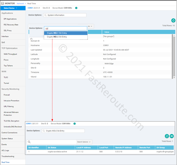
There is limited information available via real-time monitoring using vManage web interface. Native SD-WAN tunnels are also IPSec-based. These tunnels have centralized authentication and key management done by OMP instead of IKE/ISAKMP protocols used in non-SD-WAN tunnels. Real-time device options that contain string IKE in their name will be relevant to us in the context of this article.
Figure 9. Validate IKE tunnel status
Using SSH connection to the router these 2 commands can be used to check operational details of the tunnel:
show crypto isakmp sa / show crypto ikev2 sa
show crypto ipsec sa
We will demonstrate output of these commands in the practical example below.
Cisco SD-WAN IPSec Tunnels Example
Now it’s time for a practical example. We will establish an IPsec tunnel to a Cisco IOS-XE router configured to match VPN gateways settings in public clouds. For example, AWS provides sample configuration files for different platforms (see this URL). We will apply configuration from the Cisco IOS sample, and we can assume that if our router can work with it, it will work with a real AWS gateway. The configuration is slightly adjusted to use IKEv2 by replacing all isakmp commands with IKEv2-variants.
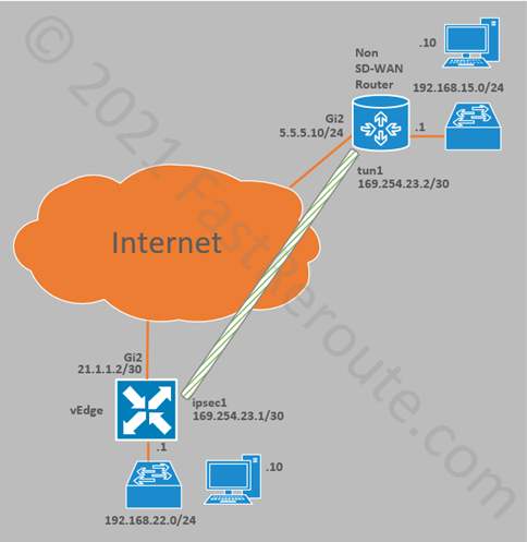
Figure 10 Cisco SD-WAN IPSec Tunnel Lab Diagram
External router configuration
Non SD-WAN router shown on the top in figure 10 has the following configuration:
interface GigabitEthernet2
 ip address 5.5.5.10 255.255.255.0

ip route 0.0.0.0 0.0.0.0 5.5.5.1

crypto ikev2 keyring KEYRING-1
 peer 21.1.1.2
  address 21.1.1.2
  pre-shared-key cisco

crypto ikev2 proposal IKE-PROPOSAL-1
 encryption aes-cbc-256
 integrity sha1
 group 16

crypto ikev2 policy IKE-POLICY-1
 match address local 5.5.5.10
 proposal IKE-PROPOSAL-1

crypto ikev2 profile IKE-PROFILE-1
 match address local interface GigabitEthernet2
 match identity remote address 21.1.1.2 255.255.255.255
 authentication remote pre-share
 authentication local pre-share
 keyring local KEYRING-1

crypto ipsec transform-set TRANSFORM-SET esp-256-aes esp-sha-hmac
 mode tunnel

crypto ipsec profile IPSEC-PROFILE-1
 set security-association lifetime kilobytes 102400000
 set transform-set TRANSFORM-SET
 set ikev2-profile IKE-PROFILE-1

interface Tunnel0
 ip address 169.254.23.2 255.255.255.252
 ip tcp adjust-mss 1400
 tunnel source GigabitEthernet2
 tunnel mode ipsec ipv4
 tunnel destination 21.1.1.2
 tunnel protection ipsec profile IPSEC-PROFILE-1

ip route 192.168.22.0 255.255.255.0 Tunnel0
SD-WAN configuration
We followed the same steps described in the first part of the article to configure vManage. To make it easier to follow, the majority of parameters are hardcoded into the template. In a real deployment, per-device variables can be used to allow for template re-use.
Then the feature template was added to the device template under VPN 1 section (see Figure 6 above) and route to 192.168.15.0/24 was added to VPN 1 feature template (see Figure 8).
Testing and Validation
Let’s assume that we have access only to the SD-WAN router, and testing will be done only from one side of the connection. We will use the router’s command-line interface via SSH from the vManage web console, as it gives access to information not available via the web interface.
The first test that we perform is checking if the remote side of the tunnel is reachable. The “vrf 1” parameter makes sure that the router uses the correct interface.
CSR01#ping vrf 1 169.254.23.2
 Type escape sequence to abort.
 Sending 5, 100-byte ICMP Echos to 169.254.23.2, timeout is 2 seconds:
 !!!!!
 Success rate is 100 percent (5/5), round-trip min/avg/max = 1/1/1 ms
 CSR01#
If ping responses are not received, we can run “show crypto ikev2 sa” and “show crypto ipsec sa” commands. The first command displays if the IKEv2 security association is established, which is a prerequisite for IPSEC security associations. The troubleshooting should start here. If IKEv1 is used, the command is “show crypto isakmp sa.”
CSR01#show crypto ikev2 sa
  IPv4 Crypto IKEv2  SA
 Tunnel-id Local                 Remote                fvrf/ivrf            Status
 1         21.1.1.2/500          5.5.5.10/500          none/1               READY
       Encr: AES-CBC, keysize: 256, PRF: SHA1, Hash: SHA96, DH Grp:16, Auth sign: PSK, Auth verify: PSK
       Life/Active Time: 86400/545 sec
 IPv6 Crypto IKEv2  SA
We were running ping of the tunnel interface in our example, which is directly connected to both routers. This test might be successful; however, the connectivity between devices behind the tunnel gateways may still not work.
In this case, we can use the “show crypto ipsec sa” command. It displays a set of counters for the number of encrypted and decrypted packets.
If the encrypted packets count is not increasing, that usually suggests a local routing problem when traffic is not being sent out of the tunnel interface.
If the encrypted packets count does increase but decrypted doesn’t, it can mean that the remote router has routing misconfiguration.
There are some useful debug commands available, such as “debug crypto ikev2”. It can generate extensive output on a router with multiple tunnels, so be careful not to overload the production router. In the example below, we’ve changed the key on the other side of the tunnel to break the tunnel. Auth exchange failed message is logged, suggesting that we have mismatched keys and “show crypto ikev2” will not display any tunnels.
CSR01#debug crypto ikev2
 Payload contents:
  VID IDi AUTH SA TSi TSr NOTIFY(INITIAL_CONTACT) NOTIFY(SET_WINDOW_SIZE) NOTIFY(ESP_TFC_NO_SUPPORT) NOTIFY(NON_FIRST_FRAGS)
 *Jul 10 00:46:36.630: IKEv2:(SESSION ID = 2,SA ID = 1):Sending Packet [To 5.5.5.10:500/From 21.1.1.2:500/VRF i0:f0]
 Initiator SPI : EE7E2D729412F370 - Responder SPI : B37D8CA8BAB8C150 Message id: 1
 IKEv2 IKE_AUTH Exchange REQUEST
 Payload contents:
  ENCR
 *Jul 10 00:46:36.633: IKEv2:(SESSION ID = 2,SA ID = 1):Received Packet [From 5.5.5.10:500/To 21.1.1.2:500/VRF i0:f0]
 Initiator SPI : EE7E2D729412F370 - Responder SPI : B37D8CA8BAB8C150 Message id: 1
 IKEv2 IKE_AUTH Exchange RESPONSE
 Payload contents:
  NOTIFY(AUTHENTICATION_FAILED)
 *Jul 10 00:46:36.633: IKEv2:(SESSION ID = 2,SA ID = 1):Process auth response notify
 *Jul 10 00:46:36.633: IKEv2-ERROR:(SESSION ID = 2,SA ID = 1):
 *Jul 10 00:46:36.633: IKEv2:(SESSION ID = 2,SA ID = 1):Auth exchange failed
 *Jul 10 00:46:36.633: IKEv2-ERROR:(SESSION ID = 2,SA ID = 1):: Auth exchange failed
 *Jul 10 00:46:36.633: IKEv2:(SESSION ID = 2,SA ID = 1):Abort exchange
 *Jul 10 00:46:36.633: IKEv2:(SESSION ID = 2,SA ID = 1):Deleting SA
 CSR01# show crypto ikev2 sa
 CSR01#
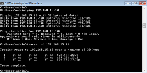
And finally we can perform end to end test from the test machines using ping and tracert commands.
This blog post describes how to enable private DNS resolution in AWS VPC, which is used internally within a VPC or from an on-premises network. We also cover different DNS integration options between AWS VPC and on-premises networks.
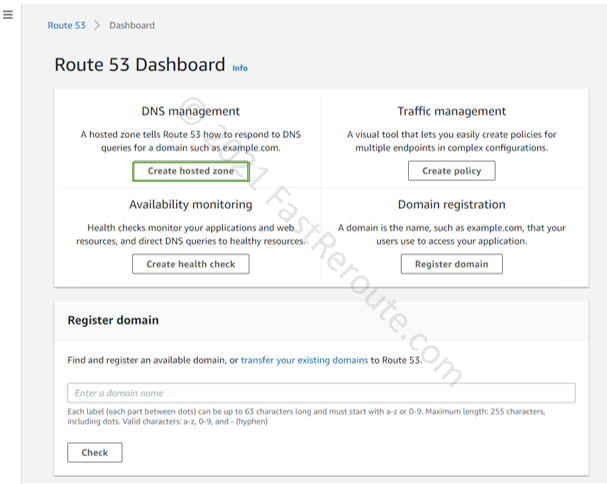
How to enable AWS Route 53 Private DNS? AWS enables Private DNS in a VPC by default. An EC2 instance is automatically assigned with a non-editable hostname derived from its private IP address in <region>.compute.internal zone. An administrator can create Route 53 private hosted zones and manually manage records in them. Private zones are not reachable from the Internet and can be assigned any domain name.
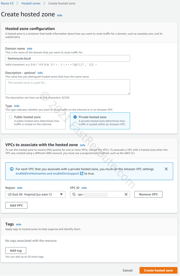
Step 2. Type in any desired domain name, select “Private hosted zone,” and choose a VPC (or VPCs) to associate this zone with. Note that AWS charges a monthly fee (not prorated for partial months) for each hosted zone. There is also a usage fee for every DNS query. AWS doesn’t charge monthly fees if the zone is deleted within 12 hours. See the detailed pricing information here.
Figure 2. Create an AWS Private Hosted Zone Detail Page
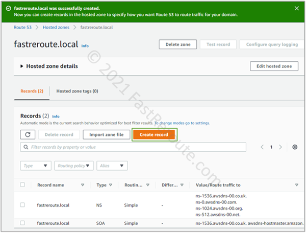
Step 3. Once the zone is created, you can add the DNS records of different types, such as A or CNAME records. Open the zone’s configuration page by clicking on it. Figure 3 shows that the private hosted zone has 2 default records – NS and SOA. Click on the Create Record button.
Figure 3. Route 53 private hosted zone overview
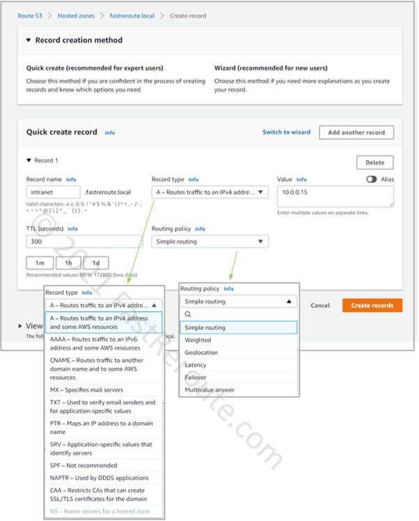
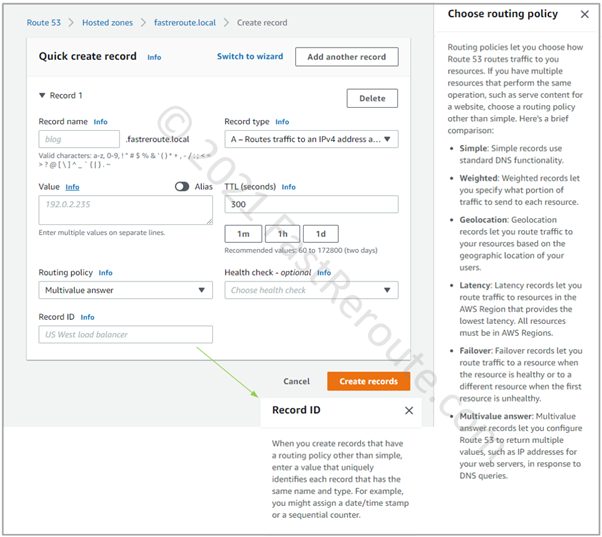
Figure 4. Create a record in AWS hosted zone
The screenshot above shows different types of records that you can create. Note that you cannot create NS records in a private hosted zone. This restricts the ability to delegate subdomains.
Step 4. Configure routing policies. AWS Route53 hosted zone can store multiple records of the same name and type. When clients try to resolve a DNS name Route 53 can reply with different values based on selected policy. Private hosted zones support only the following routing policies: simple, weighted, failover, and multivalue answer.
Routing Policies
Simple routing policy
In the previous step, we selected a simple routing policy for an A record – intranet.fastreroute.com with the value of 10.0.0.15. You can add additional IP addresses into the value textbox, as per its description label shown in the screenshot. If a query is made for intranet.fastreroute.com, the resolver will always return the same value (or values). You cannot create another A record for intranet.fastreroute.com when a simple routing policy is selected.
Multivalue routing policy
The next type of routing policy that you can use in private hosted zones is Multivalue Answer Policy. This routing policy looks up records of the same name and type and then randomly returns one.
To use this policy, create several records with the same name, for example, intranet.fastreroute.local of type A pointing to 10.0.0.15 and another one pointing to 10.0.0.16. To differentiate between these records, each must have a unique Record ID.
This feature allows performing simple DNS-based load balancing. To ensure that unreachable entries are not returned to clients, associate a health check with the record. Note that health checks rely on testing resources from outside of VPC via public IP addresses. For the resources that are not reachable externally, you can use CloudWatch alarms-based health checks instead.
Figure 5. Multivalue Answer Routing Policy
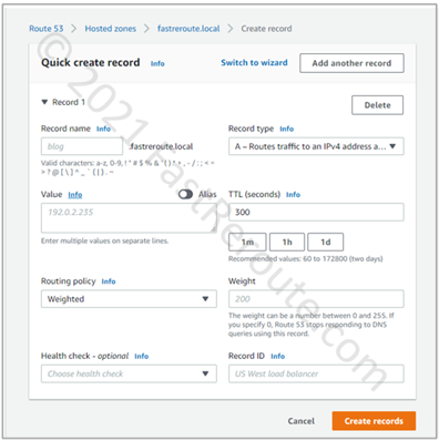
Weighted routing policy
In the screenshot below, the weighted routing policy configuration window is shown. This option load balances traffic between multiple records with the same name and type in the same way as the Multivalue answer policy. However, traffic is distributed between multiple targets not evenly but based on the relative weight. A record with a higher weight value will be returned more often than of a lower weight.
Figure 6. Weighted Routing Policy
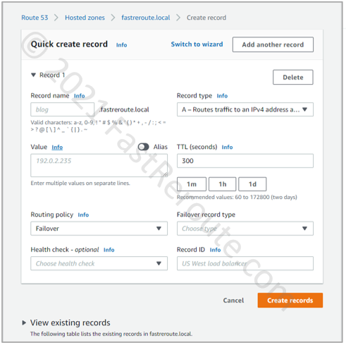
Failover routing policy
Failover routing policy example is shown in Figure 7 and enables “active/passive” routing. The policy configuration has a field called “Failover record type,” which configures one record as primary and secondary. While the primary target is healthy, its value is returned to the client. If a failure occurs with the primary target, the secondary record’s value is returned.
Figure 7. Failover Routing Policy
Step 5. Validate that the name resolution works. Testing can be performed from an EC2 instance using a VPC DNS resolver (VPC CIDR + 2). If the resolution doesn’t work, ensure that the VPC has enableDnsHostnames, and enableDnsSupport options enabled. Detailed information on how to check if these attributes are enabled is available here.
In split-view (or split-brain) DNS deployments, when the private domain name matches the public Internet domain, an internal request (for example, from EC2 instance in VPC) is matched against private hosted zones first. If no matching private hosted zone is found, the request is resolved as a public Internet query.
How to resolve entries in private hosted zones from on-premises networks?
AWS VPC Route 53 resolvers are listening on the reserved IP address of VPC CIDR + 2 and reachable internally within the VPC. However, on-premises networks connected via VPN or DirectConnect will not be able to access these resolvers directly.
Similarly, DNS requests will not flow in the reverse direction. EC2 instances within VPC often need to resolve names via on-premises DNS servers. While EC2 instances can reach on-premises servers, it is usually better to use resolvers within VPC to minimize dependence on on-premises infrastructure. Route 53 resolvers can reply to the requests for private hosted zones. However, by default, they will try to resolve all other queries via the Internet.
To address these issues, there are 2 available options:
Using an instance within VPC as DNS servers (managed by user)
Using Route 53 resolver endpoints (managed by AWS)
The following example will help to understand how these 2 options work.
Route 53 and On-premises DNS Integration Limitations
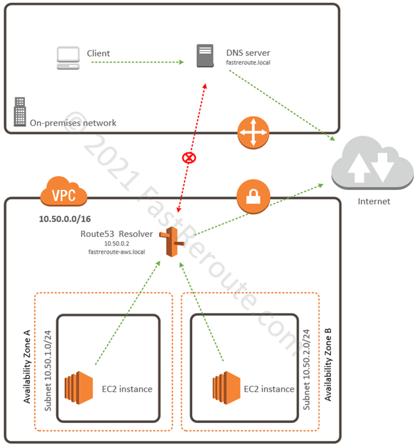
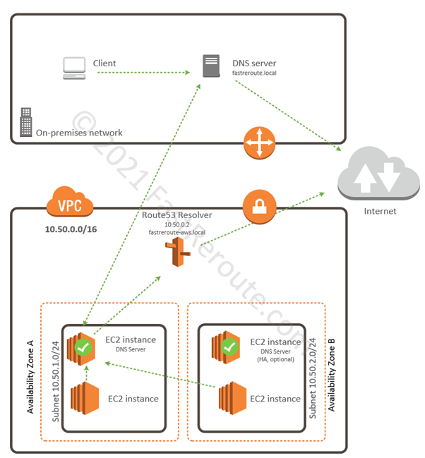
In this example, we have an internal DNS domain of fastreroute.local that is used within the corporate network. We also created a private hosted zone to use in our AWS VPC– fastreroute-aws.local.
As shown in Figure 8, the on-premises network client sends its requests to the local DNS server, which provides resolution for local zone fastreroute.local and sends all other queries to the Internet. On-premises network cannot reach Route 53 resolver, which in this example has IP address of 10.50.0.2 (VPC base prefix + 2), so we can’t forward DNS requests to the resolver by using conditional forwarding. Similarly, EC2 instances in AWS send their queries to Route 53 resolver, which can reply to queries for records in Route53 private hosted zone (fastreroute-aws.local) and forwards all non-local queries to the Internet.
Figure 8. AWS DNS Resolution Sample Diagram
User-managed DNS on EC2 instances
As briefly mentioned earlier, to enable DNS resolution to work between AWS and on-premises network, we can install an EC2 instance that will run DNS server software (it can be Windows DNS service or Linux/Unix BIND). It then can forward requests from on-premises DNS servers to Route53 resolver. You can configure EC2 instances to use it instead of using Route 53 resolver, which gives the flexibility of forwarding queries to fastreroute.local to the on-premises DNS server. Figure 9 shows how the setup works.
One of the benefits of such an approach is that it allows an organization to deploy a DNS server. For example, it can be a Microsoft AD-integrated DNS server that can support Active Directory. To provide high availability, you can deploy additional EC2 instances in a different availability zone.
Figure 9. AWS DNS Resolution using EC2 instances
AWS-managed Route 53 Endpoints
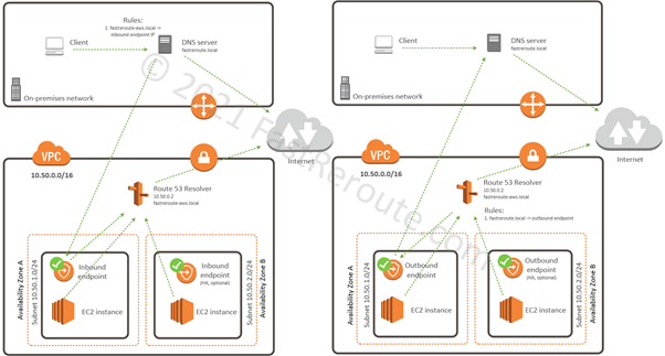
The second approach is to deploy Route 53 resolver endpoints. As shown in Figure 10, there are 2 types of resolver endpoints.
Inbound endpoints accept requests from the on-premises networks over VPN or Direct Connect. Outbound endpoints provide the way to forward DNS requests to on-premises DNS servers. Forwarding rules specify requests to which domain names are forwarded via outbound endpoint to a DNS server.
Figure 9. AWS DNS Resolution using Route 53 Inbound and Outbound Resolver Endpoints
Cisco IP Service Level Agreements (SLAs) is a proprietary feature available on Cisco routers and switches, which actively generates monitoring traffic, processes replies, and measures network performance.
This feature can be used to perform continuous end-to-end connectivity testing with automated re-routing over failover links. It can also simulate different application behavior, such as voice and video to check if the network provides the expected level of service.
The examples and features described in this article are based on Cisco IOS-XE version 16.9.
Configuration Components
IP SLA configuration starts with defining an SLA operation and then scheduling it to run immediately or at a specific time.
SLA Operation Definition
To create or edit an SLA operation use the “ip sla <operation-id>” global configuration mode command. It places CLI into the IP SLA configuration sub-mode, where you can select one of the IP SLA types and provide corresponding configuration parameters.
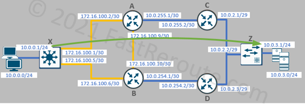
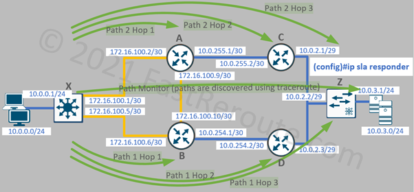
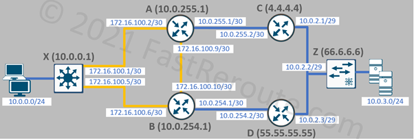
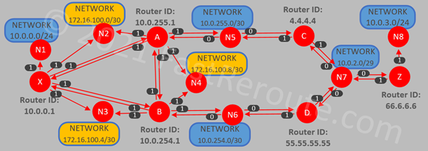
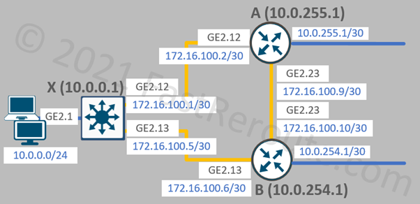
One of the simplest types of IP SLA operations is icmp-echo. The router pings a specified IP address and records round-trip times if the remote side is reachable. In the example below, we will set the type of SLA entry as ICMP echo with the destination’s IP address of 10.0.3.1. The sample topology is shown in Figure 1.
Figure 1. IP SLA Test Topology
The configuration mode changes to IP SLA echo where you can adjust different optional parameters, such as request sending frequency and timeout for replies.
X(config)#ip sla 1
X(config-ip-sla)# icmp-echo 10.0.3.1 source-ip 10.0.0.1
X(config-ip-sla-echo)#?
IP SLAs Icmp Echo Configuration Commands:
  data-pattern       Data Pattern
  default            Set a command to its defaults
  exit               Exit operation configuration
  frequency          Frequency of an operation
  history            History and Distribution Data
  no                 Negate a command or set its defaults
  owner              Owner of Entry
  request-data-size  Request data size
  tag                User defined tag
  threshold          Operation threshold in milliseconds
  timeout            Timeout of an operation
  tos                Type Of Service
  verify-data        Verify data
  vrf                Configure IP SLAs for a VRF
Scheduling IP SLA
Once SLA is defined and optional parameters are specified, start it by running the “ip sla schedule <id>” command. IP SLA can be configured to start at a specific time or as soon as the command is entered, which is shown in the example below.
X(config)#ip sla schedule 1 start-time now life forever
To check SLA operation’s details use the “show ip sla statistics <id> details” command.
X#show ip sla statistics 1 details
IPSLAs Latest Operation Statistics

IPSLA operation id: 1
        Latest RTT: 1 milliseconds
Latest operation start time: 10:08:18 UTC Sat Jan 30 2021
Latest operation return code: OK
Over thresholds occurred: FALSE
Number of successes: 2
Number of failures: 0
Operation time to live: Forever
Operational state of entry: Active
Last time this entry was reset: Never
To see configuration details, including default values for various parameters, use the “show ip sla configuration” command.
X#show ip sla configuration
IP SLAs Infrastructure Engine-III
Entry number: 1
Owner:
Tag:
Operation timeout (milliseconds): 5000
Type of operation to perform: icmp-echo
Target address/Source address: 10.0.3.1/10.0.0.1
Type Of Service parameter: 0x0
Request size (ARR data portion): 28
Data pattern: 0xABCDABCD
Verify data: No
Vrf Name:
Schedule:
   Operation frequency (seconds): 60  (not considered if randomly scheduled)
   Next Scheduled Start Time: Start Time already passed
   Group Scheduled : FALSE
   Randomly Scheduled : FALSE
   Life (seconds): Forever
   Entry Ageout (seconds): never
   Recurring (Starting Everyday): FALSE
   Status of entry (SNMP RowStatus): Active
Threshold (milliseconds): 5000
Distribution Statistics:
   Number of statistic hours kept: 2
   Number of statistic distribution buckets kept: 1
   Statistic distribution interval (milliseconds): 20
Enhanced History:
History Statistics:
   Number of history Lives kept: 0
   Number of history Buckets kept: 15
   History Filter Type: None
Once SLA operation is scheduled, it cannot be modified. Instead, the old operation can be deleted, and then a new one created again using the same ID.
Different IP SLA Types
To view available types of SLA operations, use context-sensitive help as shown in the next example.
Jitter is a variation in the delay between packets. The smaller the jitter the better performance of time-sensitive applications such as voice. It also means that the network delivers packets with a predictable delay and doesn’t experience congestions causing intermittent delays along the paths.
There are 2 types of SLA operations performing Jitter measurements – ICMP and UDP-based.
ICMP Jitter
ICMP Jitter SLA operation is based on ICMP message types (Timestamp Request and Timestamp Reply). The destination can be any device that supports these ICMP messages. Not all devices support it, or it can be blocked by the firewalls. The previously shown ICMP Echo operation is based on more commonly used Echo and Reply message types.
The configuration in the example below demonstrates how to configure ICMP jitter operation and, that once launched, it reports the round-trip-time (RTT) and jitter statistics from the source to the destination, and vice versa.
X(config)# ip sla 2
X(config-ip-sla)# icmp-jitter 10.0.3.1 source-ip 10.0.0.1
X(config)# ip sla schedule 2 start-time now life forever

X#show ip sla statistics 2
IPSLAs Latest Operation Statistics

IPSLA operation id: 2
Type of operation: icmp-jitter
        Latest RTT: 1 milliseconds
Latest operation start time: 00:20:39 UTC Sun Jan 31 2021
Latest operation return code: OK
RTT Values:
        Number Of RTT: 10               RTT Min/Avg/Max: 1/1/1 milliseconds
Latency one-way time:
        Number of Latency one-way Samples: 0
        Source to Destination Latency one way Min/Avg/Max: 0/0/0 milliseconds
        Destination to Source Latency one way Min/Avg/Max: 0/0/0 milliseconds
Jitter Time:
        Number of SD Jitter Samples: 9
        Number of DS Jitter Samples: 9
        Source to Destination Jitter Min/Avg/Max: 0/1/1 milliseconds
        Destination to Source Jitter Min/Avg/Max: 0/1/1 milliseconds
Over Threshold:
        Number Of RTT Over Threshold: 0 (0%)
Packet Late Arrival: 0
Out Of Sequence: 0
        Source to Destination: 0        Destination to Source 0
        In both Directions: 0
Packet Skipped: 0       Packet Unprocessed: 0
Packet Loss: 0
        Loss Periods Number: 0
        Loss Period Length Min/Max: 0/0
        Inter Loss Period Length Min/Max: 0/0
Number of successes: 4
Number of failures: 0
Operation time to live: Forever
To measure jitter, a source router sends a number of packets (10, by default) periodically. The time between these packets is called interval (20ms). The operation is repeated at a specified frequency (60 seconds by default).
The example below shows default configuration values – every 60 seconds the router will send 10 packets with 20 milliseconds interval between each packet.
X#show ip sla configuration 2
IP SLAs Infrastructure Engine-III
Entry number: 2
Owner:
Tag:
Operation timeout (milliseconds): 5000
Type of operation to perform: icmp-jitter
Target address/Source address: 10.0.3.1/10.0.0.1
Packet Interval (milliseconds)/Number of packets: 20/10
Type Of Service parameter: 0x0
Vrf Name:
Schedule:
   Operation frequency (seconds): 60  (not considered if randomly scheduled)
<output is truncated>
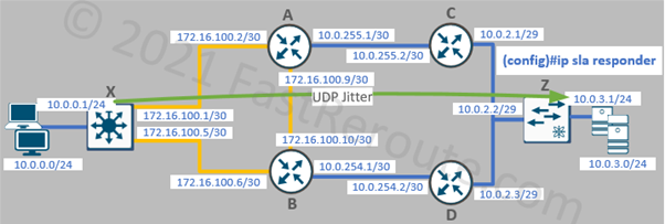
UDP Jitter and IP SLA responder
UDP is used in voice and video communications. Using UDP traffic for measurements suits better to simulate such applications. In an IP SLA operation configuration codec type can be specified, and this will define packet size and enable various voice-specific metric calculations, such as Mean Opinion Score (MOS).
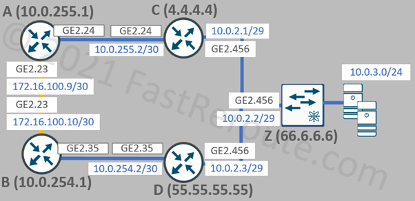
Figure 2. IP SLA Responder Configuration
To use the UDP Jitter destination device must also be a Cisco device with an IP SLA responder feature enabled on it. The responder’s basic configuration is completed with the single command on router Z:
Z(config)#ip sla responder
Back on the router X, IP SLA configuration is done per the example below.
X(config)#ip sla 3
X(config-ip-sla)#udp-jitter 10.0.3.1 2345 source-ip 10.0.0.1
X(config)#ip sla schedule 3 start-time now life forever
X#show ip sla statistics
IPSLAs Latest Operation Statistics

IPSLA operation id: 3
Type of operation: udp-jitter
        Latest RTT: 1 milliseconds
Latest operation start time: 05:53:56 UTC Sun Jan 31 2021
Latest operation return code: OK
RTT Values:
        Number Of RTT: 10               RTT Min/Avg/Max: 1/1/1 milliseconds
Latency one-way time:
        Number of Latency one-way Samples: 0
        Source to Destination Latency one way Min/Avg/Max: 0/0/0 milliseconds
        Destination to Source Latency one way Min/Avg/Max: 0/0/0 milliseconds
Jitter Time:
        Number of SD Jitter Samples: 9
        Number of DS Jitter Samples: 9
        Source to Destination Jitter Min/Avg/Max: 0/1/1 milliseconds
        Destination to Source Jitter Min/Avg/Max: 0/1/1 milliseconds
Over Threshold:
        Number Of RTT Over Threshold: 0 (0%)
Packet Loss Values:
        Loss Source to Destination: 0
        Source to Destination Loss Periods Number: 0
        Source to Destination Loss Period Length Min/Max: 0/0
        Source to Destination Inter Loss Period Length Min/Max: 0/0
        Loss Destination to Source: 0
        Destination to Source Loss Periods Number: 0
        Destination to Source Loss Period Length Min/Max: 0/0
        Destination to Source Inter Loss Period Length Min/Max: 0/0
        Out Of Sequence: 0      Tail Drop: 0
        Packet Late Arrival: 0  Packet Skipped: 0
Voice Score Values:
        Calculated Planning Impairment Factor (ICPIF): 0
        Mean Opinion Score (MOS): 0
Number of successes: 1
Number of failures: 0
Operation time to live: Forever
Path operations
When measuring latency between two hosts it is useful to know how much delay is contributed by each hop along the path. Path-type SLAs work by running traceroute first and then performing echo or jitter operation against each discovered hop.
X(config)#ip sla 4
X(config-ip-sla)#path-echo 10.0.3.1 source-ip 10.0.0.1
X(config)#ip sla schedule 4 start-time now life forever
The configuration is based on the same network topology with 2 paths available to the destination.
Figure 3. IP SLA Path Operations
The “show ip sla statistics aggregated 4 details” command will display round-trip time statistics for each hop. For example, the command output below shows statistics for the first hop in the path going via router B. The remaining hops statistics are omitted in the example below.
X#show ip sla statistics aggregated 4 details
IPSLAs aggregated statistics

Distribution Statistics:
Bucket Range: 0 to < 20 ms
Avg. Latency: 1 ms
Percent of Total Completions for this Range: 100 %
Number of Completions/Sum of Latency: 1/1
Sum of RTT squared low 32 Bits/Sum of RTT squared high 32 Bits: 1/0
Operations completed over threshold: 0
Start Time Index: *09:54:47.234 UTC Tue Feb 2 2021
Path Index: 3
Hop in Path Index: 1
Type of operation: path-echo
Number of successes: 18
Number of failures: 0
Number of over thresholds: 0
Failed Operations due to Disconnect/TimeOut/Busy/No Connection: 0/0/0/0
Failed Operations due to Internal/Sequence/Verify Error: 0/0/0
Failed Operations due to Control enable/Stats retrieve Error: 0/0
Target Address 172.16.100.6
<output is truncated>
Other operations
IP SLA can perform application-specific monitoring, for example, it can run HTTP or FTP operations against a remote server. For generic TCP applications, TCP operation can be used, which validates if the TCP connection can be established and how long it takes to connect to the server.
The other available operation types are DHCP (checks how long it takes to obtain an IP address) and DNS queries.
Reactions and Proactive Monitoring
In the previous sections, we’ve reviewed different types of SLA operations and how to check their operations using CLI. By using SNMP-based monitoring software, administrators can poll SLA data from routers periodically, which is a more scalable approach to monitoring. Cisco provides SNMP MIB called RTTMON that provides access to IP SLAs from monitoring software.
It is also possible for a router to send an SNMP trap or Syslog message if a certain event happens. IP SLA includes a feature called proactive threshold monitoring. To enable it IP SLA reaction must be configured.
The example below uses a previously configured IP SLA operation of icmp-echo type.
ip sla 1
 icmp-echo 10.0.3.1 source-ip 10.0.0.1
ip sla schedule 1 life forever start-time now
The reaction configuration below references SLA operation 1 and selects timeout as a monitored element. Then we enable simple SNMP configuration to send a trap when operations times out.
The final section of this document addresses how a router can change its data plane operation in response to IP SLA operational status.
The feature responsible for translating the status of IP SLA operations to the data plane protocols is called Enhanced Object Tracking. First-Hop Redundancy Protocols, such as HSRP and VRRP use the tracking objects to take over or release data forwarding roles. Static and policy-based routing can also use the tracking objects to re-route around degraded paths.
EEM (Embedded Event Manager) scripts can monitor tracking object’s status changes. This makes it possible to run powerful EEM scripting in response to track status change.
A Track object can have 2 states – Up and Down. IP SLA operations can have several return codes. For the purpose of object tracking, we are interested in the 3 return codes discussed below. All other codes that are not covered in this article translate into the Down state of the Track object.
Let’s re-use the IP SLA ICMP Echo operation from the previous example and check the code of the operation. The second command in the listing shows how to check the default threshold (5000ms):
X#show ip sla statistics 1 | incl code
Latest operation return code: OK
X#show ip sla configuration 1 | include Threshold
Threshold (milliseconds): 5000
The operation’s return code is OK, which means that the ping operation is successful and its round-trip time is within the threshold (in our network it is 1ms). OK status always translates to the UP state of the corresponding track object.
If we will turn off the remote interface on router Z, the return code will change to Timeout, as per the listing below. This is the second SLA operation code, which always translates into the Down state of the Track object.
The third code that is relevant for the purpose of track operation is OverThreshold. To demonstrate it, we increased the request data size to 5000 bytes, so the operation takes longer than 1ms. We also decreased the threshold to 1ms, so the operation goes over the threshold.
The OverThreshold code translates differently to the track object state, which we will discuss in the next section.
X(config)#ip sla 2
X(config-ip-sla)#icmp-echo 10.0.3.1 source-ip 10.0.0.1
X(config-ip-sla-echo)# request-data-size 5000
X(config-ip-sla-echo)# threshold 1
X(config)#ip sla schedule 2 start-time now life forever

X#show ip sla statistics 2
IPSLAs Latest Operation Statistics

IPSLA operation id: 2
        Latest RTT: 2 milliseconds
Latest operation start time: 09:44:48 UTC Sat Feb 6 2021
Latest operation return code: Over threshold
Number of successes: 2
Number of failures: 0
Operation time to live: Forever
IP SLA Track State vs. Reachability
“track <id> ip sla <sla-id>” command creates a track object that references SLA operation. There are 2 types of track objects for SLA – reachability, and state. Let’s configure both types against the previously configured SLA 2 to see the difference.
X(config)#track 1 ip sla 2 reachability
X(config)#track 2 ip sla 2 state

X#show track
Track 1
  IP SLA 2 reachability
  Reachability is Up
    1 change, last change 00:00:29
  Latest operation return code: Over threshold
  Latest RTT (millisecs) 2
Track 2
  IP SLA 2 state
  State is Down
    1 change, last change 00:00:17
  Latest operation return code: Over threshold
  Latest RTT (millisecs) 2
Track 1 is based on reachability and it is UP, even when the underlying IP SLA object is over the threshold. As the name suggests, we only interested in the fact that we can reach the remote side of the connection. Track 2 is state-based and it returns DOWN for the same IP SLA object. Track of the state type checks both reachability and that the IP SLA object is under the specified threshold.
Static Routes
The next listing demonstrates how to use the track objects with static routes:
X(config)#ip route 0.0.0.0 0.0.0.0 172.16.100.2 track 1 200
X(config)#ip route 0.0.0.0 0.0.0.0 172.16.100.6 track 2

X#sh ip route 0.0.0.0
Routing entry for 0.0.0.0/0, supernet
  Known via "static", distance 200, metric 0, candidate default path
  Routing Descriptor Blocks:
  * 172.16.100.2
      Route metric is 0, traffic share count is 1
The route via 172.16.100.6 is the preferred, as it has the default administrative distance of 1. The route via 172.16.100.2 is a backup route with an administrative distance of 200. However, the route table shows that the router prefers the route via 172.16.100.2.
For a route to be installed into the routing table the corresponding track must be UP. Because track object #2 is Down, the static route via 172.16.100.6 is withdrawn and the backup route is chosen and installed into the routing table.
EEM Scripts with IP SLA
The final example of this article is an EEM (Embedded Event Manager) script that adjusts the router configuration, generates a Syslog message in response to the Track state change.
The script is triggered when Track object #1 goes down, with the “event track <object-id> state down” command.
The access-list is being adjusted by the script in this example only for demonstration purposes. It can be adjusted to suit real-life requirements. For example, the script can reconfigure VPN tunnel endpoints or enable a backup interface. EEM can perform many other non-CLI actions as well.
To test the script, I’ve turned off the remote interface on router Z causing IP SLA and track to go down. The router generates a test Syslog message and creates an access-list, as shown in the listing below. “terminal monitor” command displays console messages into VTY lines, such as SSH or Telnet.
X#terminal monitor
*Feb  6 10:13:50.285: %TRACK-6-STATE: 1 ip sla 2 reachability Up -> Down

*Feb  6 10:13:50.530: %HA_EM-6-LOG: TRACK-1-DOWN: TEST Message

X#sh run | section ^ip access-list
ip access-list extended INTERNET-IN
 permit ip host 1.2.3.4 any
CCNA Exam (200-301) blueprint includes only a single dynamic routing protocol – OSPF (Open Shortest Path First).
The protocol is simple to enable. The basic configuration of OSPF requires only a couple of commands. However, to understand how the protocol works an exam candidate must learn OSPF components, some of them are complex. CCNA exam tests knowledge of OSPF operation in a single-area network. Multi-area components are covered in CCNP-level exams.
Routing protocols help routers to exchange reachability information and calculate the best path to the remote networks. In this blog post, we will explain how OSPF routers perform these tasks.
CCNA Exam blueprint at the time of writing comprised of the topics listed below.
The exam expects knowledge of the following facts about OSPF:
OSPF is a link-state routing protocol
OSPFv2 is the current version for IPv4; IPv6 is supported by OSPFv3
OSPF uses IP protocol number 89
2 multicast groups are reserved and used for some of the OSPFv2 protocol messages – 224.0.0.5 (AllSPFRouters) and 224.0.0.6 (AllDRRouters)
OSPF on Cisco devices has an administrative distance of 110
Overview and Basic Configuration
OSPF builds a link-state database (per area), which contains information about routers, their interfaces, and networks. The database content is synchronized across all routers.
Each router applies the Shortest Path algorithm to the database. As the result, the loop-free tree of the most efficient paths is derived. The router performing calculation is at the root of the tree having paths to every other router and network.
Initial OSPF configuration on a Cisco router uses 2 parameters:
Process ID
Router ID
Process ID
OSPF configuration starts with enabling it globally using “router ospf <process-id>” command.
The process ID is a locally significant number and doesn’t have to be the same on different routers in the network. It is possible to start several independent OSPF processes on a router, which will be assigned different process IDs.
The example below enables the OSPF process with an ID of 100 on a router. Basic router configuration, such as the assignment of IP addresses to interfaces, is omitted.
After OSPF is enabled, “show ip ospf” command confirms that the process is started.
Router# show ip ospf
Routing Process "ospf 100" with ID 10.10.10.2
<output is truncated>
Router ID
Router ID provides an identifier for an OSPF router in the form of an IPv4 address, which doesn’t need to be reachable by other OSPF routers and is not used in data forwarding. Ensure that the router ID is unique across the network. Router ID associates information with the router generating it. It is also used in multiple election processes as a tie-breaker.
As Figure 1 shows Router ID is part of the OSPF header and effectively part of every OSPF packet that the router generates.
Figure 1. OSPF Header
By default, the OSPF process will automatically assign Router ID by selecting the highest IP address of a loopback interface on the router. If there are no loopback interfaces available, then the highest IP address of a non-loopback interface is selected. As shown in Figure 2, the router has 2 physical and 2 loopback interfaces configured. Numbers are shown next to the interface name in green display the priority of interfaces for the purpose of Router ID selection.
“show ip ospf” output from the example above demonstrates that the router ID was selected to match the highest IP address of a loopback interface (10.10.10.2). The example also demonstrates that candidate interfaces for router ID selection don’t have to run OSPF.
Figure 2. OSPF Router ID Selection
Setting Router ID manually is a recommended best practice, that ensures that IDs are allocated to OSPF speakers in a pre-determined manner.
Let’s change router ID manually to 10.0.0.1.
Router(config)# router ospf 100
Router(config-router)# router-id 10.0.0.1
% OSPF: Reload or use "clear ip ospf process" command, for this to take effect
Router ID change requires the process restart. It will disrupt the packet flow, so it should be planned for in the production environment. To confirm that router ID is now adjusted let’s clear the OSPF process and then execute “show ip ospf” command.
Router# clear ip ospf 100 process
Reset OSPF process 100? [no]: yes
Router# show ip ospf
 Routing Process "ospf 100" with ID 10.0.0.1
 <output is truncated>
Link-State View of the Network
This section introduces some important concepts that will help to understand link-state advertisements (LSAs), the algorithm, and neighbor adjacencies described later in the article.
To visualize how OSPF sees a network, let’s use a sample network topology shown in Figure 3. All routers and networks are part of the same area.
Figure 3. Link-State Database Example – Full Network Diagram
Network Types
If more than 2 routers can attach to a network, it is a multi-access network, which can be divided into 3 subtypes:
Broadcast multi-access
Non-broadcast multi-access
Point-to-multipoint
A network connecting a maximum of 2 routers classified as a point-to-point network. It can be a physical point-to-point technology, or a multi-access network, such as Ethernet, administratively configured as point-to-point.
Only point-to-point and broadcast networks are listed in the blueprint of the CCNA exam. These types are commonly used and routers can auto-discover each other without any additional configuration.
For demonstration purposes, assume that yellow links (X-A, X-B, A-B) are point-to-point and blue links (A-C, B-D, C-D-Z) are multi-access broadcast networks in the sample topology shown in Figure 3.
OSPF database describes a network as a directed graph, with routers and subnets as vertices, connected to each other with the directional edges.
Let’s first re-draw the diagram displaying only routers and subnets as vertices without any connections between them.
Figure 4. Link-State Database Example – Routers and Networks as Vertices
Routers are connected bi-directionally to each other over point-to-point links, i.e. not connected via subnet vertices. We will explain how numbered point-to-point subnet vertex is connected to the routers in the next step. For now, these links are introduced between routers:
X -> A, A -> X
X -> B, B -> X
A -> B, B -> A
Transit Networks
Each multi-access broadcast network is a vertex on the graph if there are two or more routers connected to it. Such networks are called a transit and represented by vertices, which connect bi-directionally to the attached routers:
A -> N5, N5 -> A, C -> N5, N5 -> C
B -> N6, N6 -> B, D -> N6, N6 -> D
C -> N7, N7 -> C, D -> N7, N7 -> D, Z -> N7, N7 -> Z
Networks N5 and N6 have only two routers connected in this topology, however, as per our earlier assumption, the underlying data link is a multi-access broadcast network, such as Ethernet. Therefore, router pairs (A-C) and (B-D) are not connected directly as was the case on point-to-point networks. Instead, they bi-directionally connect to the transit network vertices.
Figure 5 shows the resulting connectivity.
Figure 5. Link-State Database Example – Point-to-Point and Transit Networks
Stub Networks
Finally, N1 and N8 are multi-access broadcast networks with each having only a single router connected. Both are considered to be stub networks and described by unidirectional connections from routers X and Z.
Numbered point-to-point subnets are also represented as stub networks, connected using directional link from each router: X -> N2, A -> N2, X -> N3, B -> N3, A -> N4, B -> N4. Point-to-point networks are not transit vertices, which is different to broadcast multi-access networks (N5, N6, and N7).
One of the reasons for this is that the physical point-to-point links can be unnumbered (when there are no IP addresses assigned to both sides), in which case no network vertex exists. Also, physical point-to-point links can have IPs allocated from different subnets on each side of the connection. In this case, each router has a unidirectional connection to the IP address on the other side, which are also represented as stubs.
The summary of new connections:
X -> N1
X -> N2, A -> N2
A -> N4, B -> N4
X -> N3, B -> N3
Z -> N8
Figure 6. Link-State Database Example – Stub Networks Added
Interface Cost
OSPF uses cumulative cost as the metric to compare multiple paths to the same destination. Figure 7 shows an updated diagram with associated costs displayed next to each directional edge. The cost for each vertex is calculated in the outbound direction.
Cisco routers calculate cost by dividing reference bandwidth by interface bandwidth. Consider that the reference bandwidth is 100Mbps. Interfaces of 100Mbps and higher will have a cost of 1. 10Mbps interface is 10-times slower than 100Mbps, so it will be assigned a cost of 10.
The cost value can also be manually specified using “ip ospf cost <cost-value>” interface command. As each connection between routers is represented by 2 directional edges, the cost doesn’t have to match on each side of the link. While routers connected over point-to-point links usually should have the same cost, edges from transit networks always have the cost of 0 (for example, N5 -> A).
Figure 7. Link-State Database Example – Interface Cost
Reference Bandwidth
As mentioned in the previous section, Cisco routers use reference bandwidth to calculate interface cost. “show ip ospf” command displays the reference bandwidth, which has default value of 100Mbps:
Router#show ip ospf
 <output is truncated>
 Reference bandwidth unit is 100 mbps
The virtual router that we are using in this lab has Gigabit interfaces, however, as the default reference bandwidth is 100Mbps, all interfaces with a speed higher than 100Mbps have the cost of 1.
The reference bandwidth should be adjusted on all routers in the network to match the highest bandwidth interface in the network.
Selecting Best Path
The best path within the area is calculated by each router applying the Dijkstra algorithm to its link-state database. A simplified overview of the algorithm is presented below. For more detailed information, refer to the RFC (https://tools.ietf.org/html/rfc2328#page-161).
The algorithm starts with a vertex representing the router performing the calculation. The distance to directly adjacent vertices (i.e. other routers or transit networks) is calculated and recorded in a candidate list.
The algorithm then changes the focus to the closest vertex from the candidate list. Its adjacent non-visited vertices are added to the candidate list along with their distances. The current vertex is now considered to be visited. It is removed from the candidate list and added to the shortest path.
The algorithm goes through the updated candidate list and selects the closest vertex. The process in the previous paragraph repeats till there will be no unvisited vertices left – as the result of the algorithm all reachable vertices will be added to the shortest-path tree.
After distance to all routers and transit networks is known, distances to stub networks are added via the corresponding router.
Neighbors and Adjacencies
Hello Protocol
Hello protocol is responsible for 2 tasks:
Neighbor discovery and establishment of bidirectional communication
Designated and Backup Designated Routers election on a broadcast multi-access network
OSPF routers automatically discover each other by periodically sending multicast Hello packets. On broadcast and point-to-point networks routers send Hello packets to the AllSPFRouters multicast group address (224.0.0.5).
The format of Hello packet is shown in Figure 8.
A router receiving any OSPF packet, including Hello packets, checks that Area is the same as locally configured on the router and that the authentication parameters are correct.
Then Hello-specific parameters are validated. Fields listed in the first line of the Hello packet must match between two routers to establish bidirectional communication:
Network mask must match on multi-access networks, however, is not being compared on point-to-point links.
Hello and Router Dead Intervals (in seconds) specify how often Hello packets are sent and how long other routers should wait for a Hello packet before declaring advertising router dead.
Options include a flag called E-bit. When this flag is set, the area is capable of processing External routing information, i.e. is not a stub. This flag must match between neighbors too.
Figure 8. Hello Packet
Routers include a list of neighbors on the same network segment if they have received Hello packets from them. If a router sees itself in the list of neighbors from another router it knows that bidirectional communication is established.
Neighbors go through series of states as part of Hello protocol.
Down is a state when 2 neighbors haven’t seen or stopped receiving Hello packets from each other.
In Attempt state, available only in NBMA (Non-Broadcast Multi-Access) networks, no Hello packets were received from a manually configured neighbor. The local router sends periodical unicast Hello packets to a such neighbor.
Init state means that a Hello packet has been received from the neighbor, but the router hasn’t seen itself in the list of the neighbors.
In the 2-Way state, the router receives Hello packets from the neighbor. The local router appears in the Neighbors field of these Hello packets.
Hello protocol responsibilities end when neighbors achieve the 2-Way state. Only valid neighbors will be able to reach the 2-Way state. Further stages are controlled by the Database Exchange process and routers progressing past 2-Way are referred to as adjacent routers.
On point-to-point networks, valid neighbors always become adjacent. However, on multi-access networks adjacency is established in a dual-hub-and-spokes fashion. Hubs are called a Designated Router (DR) and Backup Designated Router (BDR).
DR and BDR on Multi-Access Broadcast networks
Designated Router and Backup Designated Routers are elected on multi-access broadcast networks to decrease the number of network adjacencies required to be built (full-mesh vs dual-hub-and-spokes).
The election is based on configurable router’s interface priority and the highest router ID serves as a tie-breaker. Numerically higher priority wins. If it is set to 0, the router is not eligible to become a DR or BDR.
Hello protocol facilitates the election process by having 3 fields within the Hello packet – DR, BDR, and Router priority. If a router joins a network and receives packets with DR and BDR populated, it will not initiate the election process even if it has a better priority. This behavior is described as being non-preemptive.
Designated Router has also an important purpose – it originates Network Link State Advertisements (LSAs) representing transit network. We will discuss LSAs after we review the next stages that lead to adjacency – Database Exchange.
Database Exchange
Neighbors that have established bidirectional communication can start a process to form OSPF adjacency and synchronize their databases. As mentioned previously, routers on point-to-point links always become adjacent and routers on multi-access networks become adjacent only with DR and BDR routers.
Routers progress through a set of states before reaching a fully synchronized state:
In the Exstart state, routers decide which router will be responsible for managing the database synchronization process. Router with the highest Router ID performs the master role and its neighbor operates as a slave. OSPF Database Description packets describe LSAs that constitute each router’s database. If either neighbor sees missing or newer LSA, it will add it to the Link State Request list.
By reaching Exstart state, the routers have already progressed through all Hello protocol stages and most of the protocol parameters are found to be compatible. During the Exstart stage, theDatabase Description packet MTU field is compared with the receiving router’s interface MTU. If it doesn’t match on both sides of the adjacency, one of the routers will drop the Database Description packets. This will prevent progressing to the next stages. The behavior can be disabled on Cisco routers.
During Exchange state routers describe their link state databases by exchanging Database Description packets. The Master increments sequence numbers and waits for the Slave to acknowledge the last sequence number received from the Master.
In Loading state routers send each other Link State Request packets asking the neighbor to send LSAs that were discovered during Exchange state.
Routers in Full state are fully adjacent and have synchronized their Link State Database.
Link State Advertisements
Link State Advertisements (LSAs) describe router and network state. As reviewed in the Link-State View of the Network section earlier, OSPF sees a network as a graph of vertices connected to each other. Different types of LSAs correspond to different types of vertices, for example, a router LSA is a representation of a router vertex and a network LSA – of a transit network vertex.
We will discuss only intra-area types of LSAs (Router and Network) in this blog post. There are also other types of LSAs that exist describing inter-area and external destinations.
All LSAs share the same header. Some fields can have different values depending on the LSA type. LSA header comprises of (some of the fields are omitted in the description below and diagrams):
LSA Type. 1 is Router LSA, 2 is Network LSA
Link State ID. For Router LSA – Router ID, for Network LSA – interface IP address of the Designated Router.
Advertising Router. Router ID of the router originated LSA.
LS Age. In seconds, increments as routers transmit LSA and while it is stored in the database. Used to age out LSAs once they reach MaxAge, after which such LSAs must be re-flooded.
LS Sequence Number. Assigned by the originating router and is used for versioning of LSAs.
Router LSA
Router LSA describes the router’s links. Each link is described by several fields (not all fields are shown in the diagram and the description below):
Link ID. Depending on link type can be neighbor’s Router ID, DR’s IP address, or Network IP address.
Link Data. Depending on link type, identifies the local interface of the router or subnet mask (see mapping in the diagram below).
Figure 9. Router LSA
Network LSA
This LSA describes a multi-access network. Designated Router (DR) generates this LSA and lists all attached OSPF routers on the segment with which it formed an adjacency.
Link State ID in the header is DR’s IP address on the network. The mask is carried as a field with LSA, which makes it possible to identify the network address.
Figure 10. Network LSA
OSPF Packets
Earlier we have explored how OSPF sees the network, how routers describe their links and networks by generating LSAs that are flooded through the area. We also discussed how two routers synchronize their databases by becoming adjacent.
This section provides an overview of different types of packets that OSPF uses to distribute LSAs. Hello packet was introduced in the “Neighbors and Adjacencies” section. Figures 9 to 12 show the remaining types of OSPF packets.
Database Description packets are used during the Database Exchange process. The packet has fields describing interface MTU, various options controlling database exchange process, and sequence numbers. The payload consists of LSA headers, which format we reviewed in the previous section.
Figure 11. Database Description Packet
The next packet is the Link State Request packet. A router learns missing LSAs from received Database Description packets. To request those LSAs, the router sends a Link State Request packet which contains enough information to identify the LSA. These fields are LS Type, ID, and Advertising Router. The other LSA header fields, such as LS Age and LS Sequence Number, are not included. This means that the router is requesting the most recent version of LSA and not for the specific instance of LSA.
Figure 12. Link State Request Packet
The next 2 packets are Link State Update and Acknowledgement packets. These are used to reliably flood LSAs throughout the network. Link State Update carries a list of full LSAs with their headers.
Figure 13. Link State Update Packet
Link State Acknowledgement packet is used to explicitly confirm the receipt of a Link State Update packet.
Figure 14. Link State Acknowledgment Packet
Let’s finalize the configuration of our sample network and review different diagnostic commands.
OSPF Configuration and show commands
In this section, we will enable OSPF on different types of network interfaces using the sample topology we used earlier.
Point-to-Point Interfaces
Let’s enable OSPF between X, A, and B. In this topology, a Layer 3 LAN switch X connects to two WAN routers (A and B), which are also connected to each other.
Figure 15. Point-to-point network sample topology
Switch X configuration is shown in the listing below.
X(config)#router ospf 100
X(config-router)#network 172.16.100.0 0.0.0.3 area 0
X(config-router)#network 172.16.100.4 0.0.0.3 area 0
X(config-router)#network 10.0.0.0 0.0.0.255 area 0
network command’s purpose is to identify interfaces that will have OSPF running and which area they will be placed in. The command uses a wildcard mask, which reverses the logic of the subnet mask. In a wildcard mask, binary 0 means “match” and 1 means “ignore”.
As subnet masks use consecutive 1s followed by consecutive 0s, it can be easily converted to wildcard mask by subtracting mask value from 255.255.255.255. For example, the hostmask of 255.255.255.255 converts to a wildcard mask of 0.0.0.0.
It is possible to use a less specific wildcard mask with a network command to match multiple interfaces with a single statement. For example, instead of the 3 commands above, we could use “network 0.0.0.0 255.255.255.255 area 0”, which would enable OSPF on all interfaces and place them into area 0.
Some data-links technologies are physically point-to-point and some of them are not. As we use Ethernet in this topology, which, by default, is treated as a multi-access network additional OSPF command is required, as shown in the listing below:
There is also an alternative way to enable OSPF on interfaces available in Cisco IOS-XE. Instead of performing configuration under the OSPF process, the interface-level mode can be used. Commands in OSPF process mode are still required for global parameters, such as setting router ID. The listing below demonstrates configuration on router A, a similar configuration is also applied to router B.
“show ip ospf interface” command provides relevant to OSPF interface information. The network type of both interfaces is set to point-to-point with the cost of 1.
The next important information in the output below is the OSPF timers value. Hello timer defines how often Hello messages are sent and Dead interval specifies when the router will declare another one as dead without receiving hello messages. The values are automatically selected based on the network type or can be manually configured. Timers must match between neighbors.
In the example, hello and dead intervals have default values of 10 and 40.
X#show ip ospf interface
GigabitEthernet2.12 is up, line protocol is up
  Internet Address 172.16.100.1/30, Interface ID 13, Area 0
  Attached via Network Statement
  Process ID 100, Router ID 10.0.0.1, Network Type POINT_TO_POINT, Cost: 1
  <output truncated>
  Timer intervals configured, Hello 10, Dead 40, Wait 40, Retransmit 5
  <output truncated>
  Neighbor Count is 1, Adjacent neighbor count is 1
    Adjacent with neighbor 10.0.255.1
GigabitEthernet2.13 is up, line protocol is up
  Internet Address 172.16.100.5/30, Interface ID 14, Area 0
  Attached via Network Statement
  Process ID 100, Router ID 10.0.0.1, Network Type POINT_TO_POINT, Cost: 1
  <output truncated>
  Timer intervals configured, Hello 10, Dead 40, Wait 40, Retransmit 5
  <output truncated>
  Neighbor Count is 1, Adjacent neighbor count is 1
    Adjacent with neighbor 10.0.254.1
Interfaces were added using the router process “network <x> area <y>” configuration command, and this is indicated by the “Attached via Network Statement” line.
On routers A and B we used alternative configuration on the interface – “ip ospf <x> area <y>“. On these routers “Attached via Interface Enable” would be displayed instead.
“show ip ospf neighbors” command displays information about neighbors. Neighbor ID displays Router ID, and address specifies IP address of network interface over which neighbor is reachable. On point-to-point networks, neighbors always become adjacent and should be in FULL state. Because DR and BDRs are not elected on point-to-point networks priority value of 0 is set for both neighbors.
Deadtime is a count-down timer, which starts at 40 seconds and in normal conditions will not drop below 30 seconds, as hello packets are transmitted every 10 seconds.
X#show ip ospf neighbor
Neighbor ID     Pri   State           Dead Time   Address         Interface
10.0.254.1        0   FULL/  -        00:00:34    172.16.100.6    GigabitEthernet2.13
10.0.255.1        0   FULL/  -        00:00:39    172.16.100.2    GigabitEthernet2.12
Broadcast Multi-Access Network Interfaces
Let’s now finalize the configuration of the network topology by enabling connections between WAN routers (A <> C, B <> D), and connectivity between WAN routers C, D, and a switch Z.
Figure 16. Sample Network Diagram
The commands used for the configuration are similar to the ones shown in the previous sections. All remaining network connections are broadcast multi-access networks, which is the default OSPF network type on Ethernet interfaces. We will omit the configuration from the previous examples that set the network type to point-to-point.
Earlier, we used interface-based configuration on routers A and B. We will apply interface-level commands for additional interfaces.
A
interface Gi2.24
 ip ospf 100 area 0

B
interface Gi2.35
 ip ospf 100 area 0
For the remaining routers, we will use the router process-based configuration. For demonstration purposes, we will set router IDs as some random values to demonstrate that these addresses are neither required to be reachable over OSPF nor belong to any of the router’s interfaces. And instead of specifying individual network statements for each interface, we will use 1 wide statement that will enable OSPF on all interfaces at once.
C
router ospf 44
 router-id 4.4.4.4
 network 0.0.0.0 255.255.255.255 area 0

D
router ospf 55
 router-id 55.55.55.55
 network 0.0.0.0 255.255.255.255 area 0

Z
router ospf 66
 router-id 66.6.6.6
 network 0.0.0.0 255.255.255.255 area 0
The next example shows “show ip ospf interface” command output on router Z. Both interfaces have OSPF network type of broadcast, which is the default for Ethernet. A manually configured router ID of 66.6.6.6 is also displayed.
Z#show ip ospf interface
GigabitEthernet2.456 is up, line protocol is up
  Internet Address 10.0.2.2/29, Interface ID 12, Area 0
  Attached via Network Statement
  Process ID 66, Router ID 66.6.6.6, Network Type BROADCAST, Cost: 1
  <output truncated>
  Transmit Delay is 1 sec, State DR, Priority 1
  Designated Router (ID) 66.6.6.6, Interface address 10.0.2.2
  Backup Designated router (ID) 55.55.55.55, Interface address 10.0.2.3
  Timer intervals configured, Hello 10, Dead 40, Wait 40, Retransmit 5
  <output truncated>
  Neighbor Count is 2, Adjacent neighbor count is 2
    Adjacent with neighbor 4.4.4.4
    Adjacent with neighbor 55.55.55.55  (Backup Designated Router)
GigabitEthernet2.2 is up, line protocol is up
  Internet Address 10.0.3.1/24, Interface ID 11, Area 0
  Attached via Network Statement
  Process ID 66, Router ID 66.6.6.6, Network Type BROADCAST, Cost: 1
  <output truncated>
  Transmit Delay is 1 sec, State DR, Priority 1
  Designated Router (ID) 66.6.6.6, Interface address 10.0.3.1
  No backup designated router on this network
  Timer intervals configured, Hello 10, Dead 40, Wait 40, Retransmit 5
  <output truncated>
  Neighbor Count is 0, Adjacent neighbor count is 0
“State DR” means that the router performs the role of the Designated Router on the network segment. Backup DR will have a state listed as BDR, and all other routers will be in DROTHER state. “Priority 1” is the default priority, so the router with the highest Router ID is elected as DR if all routers start at the same time. As the process is not preemptive, the role of DR can be performed by the router with a smaller priority or Router ID value if it starts before other routers.
Information about Designated Router and Backup Designated Routers is displayed next, followed by Hello and Dead timer settings.
The last lines of output list information about neighbors and adjacencies on the interface. Both DR and BDR become adjacent with all neighbors on the network. Routers that are neither DR nor BDR will display all routers on the segment as neighbors, however, establish adjacencies only with DR and BDR.
Link State Database
In this section, we will explore the link state database on router Z.
“show ip ospf database” command displays the content of the database. For the purpose of CCNA exam preparation, the example focuses on a single-area topology.
Z#show ip ospf database

            OSPF Router with ID (66.6.6.6) (Process ID 66)

                Router Link States (Area 0)

Link ID         ADV Router      Age         Seq#       Checksum Link count
4.4.4.4         4.4.4.4         64          0x80000014 0x00EFCE 2
10.0.0.1        10.0.0.1        1655        0x80000005 0x00F639 5
10.0.254.1      10.0.254.1      116         0x8000000A 0x00B55B 5
10.0.255.1      10.0.255.1      336         0x80000007 0x00DE3B 5
55.55.55.55     55.55.55.55     64          0x80000011 0x00B077 2
66.6.6.6        66.6.6.6        208         0x8000000C 0x0071D4 2

                Net Link States (Area 0)

Link ID         ADV Router      Age         Seq#       Checksum
10.0.2.1        4.4.4.4         209         0x80000002 0x00C617
10.0.254.1      10.0.254.1      300         0x80000001 0x00C27F
10.0.255.1      10.0.255.1      1730        0x80000002 0x00B753
Router LSA
Each router generates a Router LSA, with Link ID matching the generating router’s ID. 6 LSAs are displayed matching number of routers in our topology. To understand link count, review the previous section called “Link-State View of the Network” and Figure 6, where each outbound arrow from a router is counted as a link.
For example, let’s review in detail the content of router LSA with ID 10.0.255.1 (Router A). Below is part of Figure 6 focusing on router A.
Figure 17. Router LSA Example Topology
“show ip ospf database router <router-id>” command displays detailed information about router LSA. As the link-state database is the same on all routers we can gather output on any routers in the same area. In the example below, the command is launched on router Z.
Z#show ip ospf database router 10.0.255.1

            OSPF Router with ID (66.6.6.6) (Process ID 66)

                Router Link States (Area 0)

  LS age: 142
  Options: (No TOS-capability, DC)
  LS Type: Router Links
  Link State ID: 10.0.255.1
  Advertising Router: 10.0.255.1
  LS Seq Number: 80000006
  Checksum: 0xE03A
  Length: 84
  Number of Links: 5

    Link connected to: a Transit Network
     (Link ID) Designated Router address: 10.0.255.1
     (Link Data) Router Interface address: 10.0.255.1
      Number of MTID metrics: 0
       TOS 0 Metrics: 1

    Link connected to: another Router (point-to-point)
     (Link ID) Neighboring Router ID: 10.0.254.1
     (Link Data) Router Interface address: 172.16.100.9
      Number of MTID metrics: 0
       TOS 0 Metrics: 1

    Link connected to: a Stub Network
     (Link ID) Network/subnet number: 172.16.100.8
     (Link Data) Network Mask: 255.255.255.252
      Number of MTID metrics: 0
       TOS 0 Metrics: 1

    Link connected to: another Router (point-to-point)
     (Link ID) Neighboring Router ID: 10.0.0.1
     (Link Data) Router Interface address: 172.16.100.2
      Number of MTID metrics: 0
       TOS 0 Metrics: 1

    Link connected to: a Stub Network
     (Link ID) Network/subnet number: 172.16.100.0
     (Link Data) Network Mask: 255.255.255.252
      Number of MTID metrics: 0
       TOS 0 Metrics: 1
The links in the output are shown in the following order:
A -> N5 (A is BDR on this network, so the output displays its own IP address as DR)
A -> B (A has point-to-point connectivity to B over N4; this is described by this link and additional link from A to N4 listed below)
A -> N4 (numbered subnet for the point-to-point link is represented as a connection to a stub network)
A -> X
A -> N2
Network LSA
The next example focuses on the network LSA which represents a transit network. To display network LSA, run “show ip ospf database network <id>” command. For this example, we will use the N7 network (10.0.2.0/29) connecting routers C, D, and Z.
Figure 18. Network LSA Example Topology
Network LSA ID matches the IP address of Designated Router (router Z) on this network and it lists router IDs of attached routers. The output shows routers Z, C, and D as attached to N7.
Z#show ip ospf database network 10.0.2.2

            OSPF Router with ID (66.6.6.6) (Process ID 66)

                Net Link States (Area 0)

  LS age: 1435
  Options: (No TOS-capability, DC)
  LS Type: Network Links
  Link State ID: 10.0.2.2 (address of Designated Router)
  Advertising Router: 66.6.6.6
  LS Seq Number: 80000002
  Checksum: 0x7325
  Length: 36
  Network Mask: /29
        Attached Router: 66.6.6.6
        Attached Router: 4.4.4.4
        Attached Router: 55.55.55.55
Network mask (/29) is also stored as part of the network LSA, which together with Link State ID represented by DR’s IP address can be used to obtain network IP prefix – 10.0.2.0/29.
represented by DR’s IP address can be used to obtain network IP prefix – 10.0.2.0/29.
Self-Test Questions
How OSPF router ID is selected if it's not manually configured?
The highest IP address on a loopback interface. If there are no loopback interfaces, select the highest IP address assigned to a physical interface.
What OSPF uses to compare multiple paths to a destination?
By combining costs of interfaces through each path. Each interface’s cost reflects how many times its bandwidth is smaller than a reference bandwidth. If interface speed is faster or the same as the reference value, then 1 is used as cost.
What is the difference between neighbors and adjacent routers?
Neighbors are the router that can communicate with each other and have matching parameters. Adjacency is formed between neighbors for the purpose of exchanging routing information. On multi-access networks, some of the neighbors don’t establish adjacency between each other.
What are 2 main tasks of OSPF Hello protocol?
Neighbor discovery and DR election
Explain what is router and network LSAs?
Link State Advertisement is a unit of information that is stored in each router’s Link State Database. Each router LSA represents a router and its links. Network LSA describes a transit network and lists routers connected to it.
Azure Network Security Groups (NSGs) can be complex to configure and troubleshoot. We will try to explain how they work, what components they consist of, and how to manage them.
Microsoft Certified Azure Administrator Associate Exam (AZ-104) expects good knowledge of the topics in the list below.
create security rules
associate an NSG to a subnet or network interface
evaluate effective security rules
The exam groups these topics under “Secure access to virtual networks” section along with Azure Bastion and Azure Firewall, which we will not cover in this article.
This blog post provides an overview of Azure security concepts such as NSGs and security rules, as well as practical step-by-step examples of how to implement and validate their configuration.
An administrator can protect Azure resources by applying a Network Security Group (NSG) to a network interface or a subnet.
Figure 1 shows components of a Network Security Group.
Each security rule consists of the following fields:
Rule name and description
Priority number, which defines a position of the rule in the ruleset. Rules on the top are processed first, therefore, the smaller number has a higher preference
Source and destination with port numbers (for TCP and UDP)
IP protocol type, such as TCP, UDP, and ICMP. These 3 protocols cover almost all application requirements. “Any” keyword permits all IP protocols
Figure 1. Azure Network Security Group
A Network Security Group can be applied to a network interface and to a Subnet. Applying an NSG to a Subnet simplifies the rule management if all VMs in the subnet requires the same security rules.
There is a common incorrect understanding that Subnet-level NSGs work as ACLs on a default gateway device (such as a switch or a firewall) in a traditional network, which protects traffic as it enters subnet and doesn’t check connectivity within a subnet. Subnet level NSGs should be treated as a template mechanism, they do affect traffic between VMs in the same subnet.
If no NSG is applied, then all traffic is allowed to and from a virtual machine.
Microsoft recommends applying an NSG to either interface or subnet, but not to both.
As the diagram above shows, a single NSG can associate with multiple network interfaces and subnets. Each network interface or subnet can have 0 or 1 NSGs associated with it.
Inbound vs Outbound
An NSG contains two ordered lists of Security Rules – inbound and outbound.
NSG ruleset direction is evaluated from a VM perspective. For example, rules in inbound direction affect traffic that is being initiated from external sources, such as the Internet or another VM, to a virtual machine. Outbound security rules affect traffic sent from a VM.
Return traffic for an established session is automatically allowed and is not validated against rules in the reverse direction. So we only need to focus on allowing (or denying) client-to-server direction of the session.
Default Security Rules
There are 6 default inbound (3) and outbound (3) rules that exist in each NSG. They cannot be removed or edited. An administrator can create custom rules to override the default ones.
Figure 2 extends the conceptual diagram shown in Figure 1 by adding the default rules. In addition to custom rules that users can define shown on the left side, the additional 3 rules can be seen.
The first default rule with priority (or sequence number) of 65000 allows internal communication. It permits the traffic with the source and destination IP prefixes identified by a service tag called VirtualNetwork.
VirtualNetwork service tag includes IP addresses of:
Local VNet address space
Peered VNets’ address space (configurable, see this link for details)
Address space of VNets connected to Virtual Network Gateway
User-defined routes
On-premises address spaces
and a default route (this can make NSG become “permit any” if, for example, the default route is advertised from the on-premises network)
The second rule in inbound security ruleset allows access from Azure Load Balancer to any destination. In the outbound security ruleset, the rule with the same sequence number of 65001 allows unrestricted access to the Internet.
The very last default rule in both inbound and outbound rulesets is the “Deny all” rule. It means that if there are no “allow” rules that match the specific traffic, it will be dropped.
Figure 2. Azure NSG – Default Security Rules
Evaluation Order
A packet is compared sequentially against each security rule until the first match is found. The further rules are not processed and the action in the matching rule is applied.
If an NSG is applied to a subnet and another one to a network interface, then both NSGs are processed. Subnet NSG is processed first. If a packet hits deny rule, including the default “Deny Any” rule, then the packet is dropped straight away. If the packet is allowed by subnet NSG, then the network interface’s NSG is evaluated.
NSG and Security Rules Step-by-Step Configuration
To create a Network Security Group start typing “network security” in the search bar and select Network security groups in the list of Azure services.
Create a new NSG
In the Network Security Groups window, press Add to create an NSG. Select a Resource Group and a name for NSG and press Review + Create button, as shown in Figure 3.
Figure 3. Create Azure Network Security Group
Once NSG is created, it will appear in the list shown in the upper part of Figure 3. Click on NSG to display its properties. As the screenshot below shows, the overview window of NSG-A provides summary information, as well as inbound and outbound security rule content.
NSG configuration menu provides access to:
Inbound security rules management
Outbound security rules management
Network interfaces to create an association with the NSG. This operation can also be performed via Network interface configuration pages
Subnets to create an association with the NSG. This operation can also be performed via VNet > Subnet menu configuration
Effective security rules display
Figure 4. Create Azure Network Security Group
Modify Security Rules in NSG
During VM provisioning new NSG can be automatically created with the common management ports, such as RDP and SSH, as shown in Figure 5.
Figure 5. VM Inbound Port Rule
For this example, let’s assume that an administrator didn’t select any of the ports and we cannot connect to the VM remotely. To address this issue we will use NSG created in the previous step, allow RDP, and associate the NSG with the VM’s NIC.
To add a new inbound security rule, click on the menu (#1). Then press Add (#2). Fill the information, as shown in the screenshot below, and press Add.
Figure 6. NSG Inbound Security Rules
Associate NSG with a Network Interface
In the next step, we will associate the NSG with the network interface of the VM, as shown in Figure 7. To enable this, within the NSG configuration window, click on the Network interfaces side menu (#1) and press the Associate button (#2) and select the network interface.
Figure 7. Select Network Interface via NSG Configuration Page
In some cases, the network interface will be greyed out. If this is the case, the configuration can be performed from the Network Interface configuration window. Navigate to the network interfaces list and select the one that you want to change NSG for. Choose the Network security group menu (#1) and select choose the NSG that we created earlier.
Figure 8. Associate NSG with Network Interface
Associate NSG with a Subnet
As with the Network Adapter association, the configuration can be performed via the properties of NSG or from the Subnet configuration page. To associate with a subnet via NSG properties, open Subnets menu and click on Associate and then select the virtual network and the subnet as shown in Figure 9.
In this example, we have an NSG called NSG-A-SUBNET created earlier, which we will associate with the subnet.
Figure 9. Associate Subnet via NSG Properties
To perform the same procedure using Subnet properties, navigate to the subnet configuration page via its parent VNet. Then select a Network security group drop-down box and choose the NSG.
Figure 10. Set NSG via Subnet Properties
View Effective Security Rules
Azure Network Interface properties have a button called “Effective security rules”. To be able to display this page the virtual machine that has the interface attached must be powered on.
The opened window doesn’t display rules correctly currently, as shown in Figure 11. For example, we have RDP port opened inbound on both network interface and subnet level, which is not shown in the list of rules.
This page, however, allows us to download ruleset in CSV format, so an administrator can use Excel or some automation tool to analyze it. As shown in Figure 11, we can see our RDP rules, as well as expanded service tags. For example, we can see which IP addresses are included in the Virtual Network service tag.
Figure 11. Display Effective Security Rules
The other way to check what rules are currently applied at different levels is to use the Networking properties of a VM, as shown in Figure 12. Notice how this page correctly displays subnet-level and network interface-level rules.
Figure 12. Display Effective Security Rules via VM Networking Properties
Network Security Group (NSG) is an Azure configuration element that contains a set of network-level security rules which restrict traffic from and to Virtual Machines
How a Network Security Group is applied?
An NSG can be applied either to Network Interface or to Subnet. It can be applied to both simultaneously, but it is not recommended
How many NSGs can be applied to a single Network Interface?