Configure and Verify Single Area OSPFv2
CCNA Exam (200-301) blueprint includes only a single dynamic routing protocol – OSPF (Open Shortest Path First).
The protocol is simple to enable. The basic configuration of OSPF requires only a couple of commands. However, to understand how the protocol works an exam candidate must learn OSPF components, some of them are complex. CCNA exam tests knowledge of OSPF operation in a single-area network. Multi-area components are covered in CCNP-level exams.
Routing protocols help routers to exchange reachability information and calculate the best path to the remote networks. In this blog post, we will explain how OSPF routers perform these tasks.
CCNA Exam blueprint at the time of writing comprised of the topics listed below.
3.4 Configure and verify single area OSPFv2
- 3.4.a Neighbor adjacencies
- 3.4.b Point-to-point
- 3.4.c Broadcast (DR/BDR selection)
- 3.4.d Router ID
Introduction
OSPFv2 is an open standard documented in several IETF RFCs. The current revision is RFC 2328 (https://tools.ietf.org/html/rfc2328).
The exam expects knowledge of the following facts about OSPF:
- OSPF is a link-state routing protocol
- OSPFv2 is the current version for IPv4; IPv6 is supported by OSPFv3
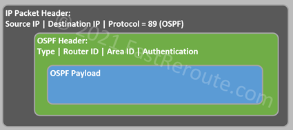
- OSPF uses IP protocol number 89
- 2 multicast groups are reserved and used for some of the OSPFv2 protocol messages – 224.0.0.5 (AllSPFRouters) and 224.0.0.6 (AllDRRouters)
- OSPF on Cisco devices has an administrative distance of 110
Overview and Basic Configuration
OSPF builds a link-state database (per area), which contains information about routers, their interfaces, and networks. The database content is synchronized across all routers.
Each router applies the Shortest Path algorithm to the database. As the result, the loop-free tree of the most efficient paths is derived. The router performing calculation is at the root of the tree having paths to every other router and network.
Initial OSPF configuration on a Cisco router uses 2 parameters:
- Process ID
- Router ID
Process ID
OSPF configuration starts with enabling it globally using “router ospf <process-id>” command.
The process ID is a locally significant number and doesn’t have to be the same on different routers in the network. It is possible to start several independent OSPF processes on a router, which will be assigned different process IDs.
The example below enables the OSPF process with an ID of 100 on a router. Basic router configuration, such as the assignment of IP addresses to interfaces, is omitted.
Router(config)# router ospf 100
Router(config-router)#
After OSPF is enabled, “show ip ospf” command confirms that the process is started.
Router# show ip ospf
 Routing Process "ospf 100" with ID 10.10.10.2
 <output is truncated>
Router ID
Router ID provides an identifier for an OSPF router in the form of an IPv4 address, which doesn’t need to be reachable by other OSPF routers and is not used in data forwarding. Ensure that the router ID is unique across the network. Router ID associates information with the router generating it. It is also used in multiple election processes as a tie-breaker.
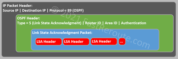
As Figure 1 shows Router ID is part of the OSPF header and effectively part of every OSPF packet that the router generates.
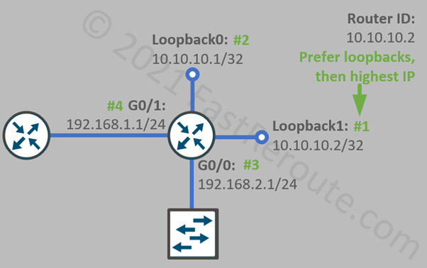
By default, the OSPF process will automatically assign Router ID by selecting the highest IP address of a loopback interface on the router. If there are no loopback interfaces available, then the highest IP address of a non-loopback interface is selected. As shown in Figure 2, the router has 2 physical and 2 loopback interfaces configured. Numbers are shown next to the interface name in green display the priority of interfaces for the purpose of Router ID selection.
“show ip ospf” output from the example above demonstrates that the router ID was selected to match the highest IP address of a loopback interface (10.10.10.2). The example also demonstrates that candidate interfaces for router ID selection don’t have to run OSPF.
Setting Router ID manually is a recommended best practice, that ensures that IDs are allocated to OSPF speakers in a pre-determined manner.
Let’s change router ID manually to 10.0.0.1.
Router(config)# router ospf 100
Router(config-router)# router-id 10.0.0.1
% OSPF: Reload or use "clear ip ospf process" command, for this to take effect
Router ID change requires the process restart. It will disrupt the packet flow, so it should be planned for in the production environment. To confirm that router ID is now adjusted let’s clear the OSPF process and then execute “show ip ospf” command.
Router# clear ip ospf 100 process
Reset OSPF process 100? [no]: yes
Router# show ip ospf
 Routing Process "ospf 100" with ID 10.0.0.1
 <output is truncated>
Link-State View of the Network
This section introduces some important concepts that will help to understand link-state advertisements (LSAs), the algorithm, and neighbor adjacencies described later in the article.
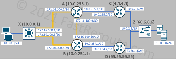
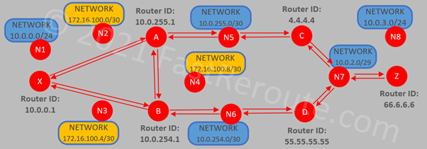
To visualize how OSPF sees a network, let’s use a sample network topology shown in Figure 3. All routers and networks are part of the same area.
Network Types
If more than 2 routers can attach to a network, it is a multi-access network, which can be divided into 3 subtypes:
- Broadcast multi-access
- Non-broadcast multi-access
- Point-to-multipoint
A network connecting a maximum of 2 routers classified as a point-to-point network. It can be a physical point-to-point technology, or a multi-access network, such as Ethernet, administratively configured as point-to-point.
Only point-to-point and broadcast networks are listed in the blueprint of the CCNA exam. These types are commonly used and routers can auto-discover each other without any additional configuration.
For demonstration purposes, assume that yellow links (X-A, X-B, A-B) are point-to-point and blue links (A-C, B-D, C-D-Z) are multi-access broadcast networks in the sample topology shown in Figure 3.
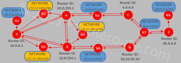
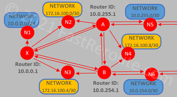
OSPF database describes a network as a directed graph, with routers and subnets as vertices, connected to each other with the directional edges.
Let’s first re-draw the diagram displaying only routers and subnets as vertices without any connections between them.

Routers are connected bi-directionally to each other over point-to-point links, i.e. not connected via subnet vertices. We will explain how numbered point-to-point subnet vertex is connected to the routers in the next step. For now, these links are introduced between routers:
- X -> A, A -> X
- X -> B, B -> X
- A -> B, B -> A
Transit Networks
Each multi-access broadcast network is a vertex on the graph if there are two or more routers connected to it. Such networks are called a transit and represented by vertices, which connect bi-directionally to the attached routers:
- A -> N5, N5 -> A, C -> N5, N5 -> C
- B -> N6, N6 -> B, D -> N6, N6 -> D
- C -> N7, N7 -> C, D -> N7, N7 -> D, Z -> N7, N7 -> Z
Networks N5 and N6 have only two routers connected in this topology, however, as per our earlier assumption, the underlying data link is a multi-access broadcast network, such as Ethernet. Therefore, router pairs (A-C) and (B-D) are not connected directly as was the case on point-to-point networks. Instead, they bi-directionally connect to the transit network vertices.
Figure 5 shows the resulting connectivity.
Stub Networks
Finally, N1 and N8 are multi-access broadcast networks with each having only a single router connected. Both are considered to be stub networks and described by unidirectional connections from routers X and Z.
Numbered point-to-point subnets are also represented as stub networks, connected using directional link from each router: X -> N2, A -> N2, X -> N3, B -> N3, A -> N4, B -> N4. Point-to-point networks are not transit vertices, which is different to broadcast multi-access networks (N5, N6, and N7).
One of the reasons for this is that the physical point-to-point links can be unnumbered (when there are no IP addresses assigned to both sides), in which case no network vertex exists. Also, physical point-to-point links can have IPs allocated from different subnets on each side of the connection. In this case, each router has a unidirectional connection to the IP address on the other side, which are also represented as stubs.
The summary of new connections:
- X -> N1
- X -> N2, A -> N2
- A -> N4, B -> N4
- X -> N3, B -> N3
- Z -> N8
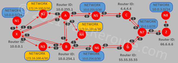
Interface Cost
OSPF uses cumulative cost as the metric to compare multiple paths to the same destination. Figure 7 shows an updated diagram with associated costs displayed next to each directional edge. The cost for each vertex is calculated in the outbound direction.
Cisco routers calculate cost by dividing reference bandwidth by interface bandwidth. Consider that the reference bandwidth is 100Mbps. Interfaces of 100Mbps and higher will have a cost of 1. 10Mbps interface is 10-times slower than 100Mbps, so it will be assigned a cost of 10.
The cost value can also be manually specified using “ip ospf cost <cost-value>” interface command. As each connection between routers is represented by 2 directional edges, the cost doesn’t have to match on each side of the link. While routers connected over point-to-point links usually should have the same cost, edges from transit networks always have the cost of 0 (for example, N5 -> A).
Reference Bandwidth
As mentioned in the previous section, Cisco routers use reference bandwidth to calculate interface cost. “show ip ospf” command displays the reference bandwidth, which has default value of 100Mbps:
Router#show ip ospf
 <output is truncated>
 Reference bandwidth unit is 100 mbps
The virtual router that we are using in this lab has Gigabit interfaces, however, as the default reference bandwidth is 100Mbps, all interfaces with a speed higher than 100Mbps have the cost of 1.
The reference bandwidth should be adjusted on all routers in the network to match the highest bandwidth interface in the network.
Selecting Best Path
The best path within the area is calculated by each router applying the Dijkstra algorithm to its link-state database. A simplified overview of the algorithm is presented below. For more detailed information, refer to the RFC (https://tools.ietf.org/html/rfc2328#page-161).
The algorithm starts with a vertex representing the router performing the calculation. The distance to directly adjacent vertices (i.e. other routers or transit networks) is calculated and recorded in a candidate list.
The algorithm then changes the focus to the closest vertex from the candidate list. Its adjacent non-visited vertices are added to the candidate list along with their distances. The current vertex is now considered to be visited. It is removed from the candidate list and added to the shortest path.
The algorithm goes through the updated candidate list and selects the closest vertex. The process in the previous paragraph repeats till there will be no unvisited vertices left – as the result of the algorithm all reachable vertices will be added to the shortest-path tree.
After distance to all routers and transit networks is known, distances to stub networks are added via the corresponding router.
Neighbors and Adjacencies
Hello Protocol
Hello protocol is responsible for 2 tasks:
- Neighbor discovery and establishment of bidirectional communication
- Designated and Backup Designated Routers election on a broadcast multi-access network
OSPF routers automatically discover each other by periodically sending multicast Hello packets. On broadcast and point-to-point networks routers send Hello packets to the AllSPFRouters multicast group address (224.0.0.5).
The format of Hello packet is shown in Figure 8.
A router receiving any OSPF packet, including Hello packets, checks that Area is the same as locally configured on the router and that the authentication parameters are correct.
Then Hello-specific parameters are validated. Fields listed in the first line of the Hello packet must match between two routers to establish bidirectional communication:
- Network mask must match on multi-access networks, however, is not being compared on point-to-point links.
- Hello and Router Dead Intervals (in seconds) specify how often Hello packets are sent and how long other routers should wait for a Hello packet before declaring advertising router dead.
- Options include a flag called E-bit. When this flag is set, the area is capable of processing External routing information, i.e. is not a stub. This flag must match between neighbors too.
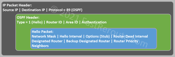
Routers include a list of neighbors on the same network segment if they have received Hello packets from them. If a router sees itself in the list of neighbors from another router it knows that bidirectional communication is established.
Neighbors go through series of states as part of Hello protocol.
- Down is a state when 2 neighbors haven’t seen or stopped receiving Hello packets from each other.
- In Attempt state, available only in NBMA (Non-Broadcast Multi-Access) networks, no Hello packets were received from a manually configured neighbor. The local router sends periodical unicast Hello packets to a such neighbor.
- Init state means that a Hello packet has been received from the neighbor, but the router hasn’t seen itself in the list of the neighbors.
- In the 2-Way state, the router receives Hello packets from the neighbor. The local router appears in the Neighbors field of these Hello packets. Hello protocol responsibilities end when neighbors achieve the 2-Way state. Only valid neighbors will be able to reach the 2-Way state. Further stages are controlled by the Database Exchange process and routers progressing past 2-Way are referred to as adjacent routers.
On point-to-point networks, valid neighbors always become adjacent. However, on multi-access networks adjacency is established in a dual-hub-and-spokes fashion. Hubs are called a Designated Router (DR) and Backup Designated Router (BDR).
DR and BDR on Multi-Access Broadcast networks
Designated Router and Backup Designated Routers are elected on multi-access broadcast networks to decrease the number of network adjacencies required to be built (full-mesh vs dual-hub-and-spokes).
The election is based on configurable router’s interface priority and the highest router ID serves as a tie-breaker. Numerically higher priority wins. If it is set to 0, the router is not eligible to become a DR or BDR.
Hello protocol facilitates the election process by having 3 fields within the Hello packet – DR, BDR, and Router priority. If a router joins a network and receives packets with DR and BDR populated, it will not initiate the election process even if it has a better priority. This behavior is described as being non-preemptive.
Designated Router has also an important purpose – it originates Network Link State Advertisements (LSAs) representing transit network. We will discuss LSAs after we review the next stages that lead to adjacency – Database Exchange.
Database Exchange
Neighbors that have established bidirectional communication can start a process to form OSPF adjacency and synchronize their databases. As mentioned previously, routers on point-to-point links always become adjacent and routers on multi-access networks become adjacent only with DR and BDR routers.
Routers progress through a set of states before reaching a fully synchronized state:
- In the Exstart state, routers decide which router will be responsible for managing the database synchronization process. Router with the highest Router ID performs the master role and its neighbor operates as a slave. OSPF Database Description packets describe LSAs that constitute each router’s database. If either neighbor sees missing or newer LSA, it will add it to the Link State Request list.
- By reaching Exstart state, the routers have already progressed through all Hello protocol stages and most of the protocol parameters are found to be compatible. During the Exstart stage, the Database Description packet MTU field is compared with the receiving router’s interface MTU. If it doesn’t match on both sides of the adjacency, one of the routers will drop the Database Description packets. This will prevent progressing to the next stages. The behavior can be disabled on Cisco routers.
- During Exchange state routers describe their link state databases by exchanging Database Description packets. The Master increments sequence numbers and waits for the Slave to acknowledge the last sequence number received from the Master.
- In Loading state routers send each other Link State Request packets asking the neighbor to send LSAs that were discovered during Exchange state.
- Routers in Full state are fully adjacent and have synchronized their Link State Database.
Link State Advertisements
Link State Advertisements (LSAs) describe router and network state. As reviewed in the Link-State View of the Network section earlier, OSPF sees a network as a graph of vertices connected to each other. Different types of LSAs correspond to different types of vertices, for example, a router LSA is a representation of a router vertex and a network LSA – of a transit network vertex.
We will discuss only intra-area types of LSAs (Router and Network) in this blog post. There are also other types of LSAs that exist describing inter-area and external destinations.
All LSAs share the same header. Some fields can have different values depending on the LSA type. LSA header comprises of (some of the fields are omitted in the description below and diagrams):
- LSA Type. 1 is Router LSA, 2 is Network LSA
- Link State ID. For Router LSA – Router ID, for Network LSA – interface IP address of the Designated Router.
- Advertising Router. Router ID of the router originated LSA.
- LS Age. In seconds, increments as routers transmit LSA and while it is stored in the database. Used to age out LSAs once they reach MaxAge, after which such LSAs must be re-flooded.
- LS Sequence Number. Assigned by the originating router and is used for versioning of LSAs.
Router LSA
Router LSA describes the router’s links. Each link is described by several fields (not all fields are shown in the diagram and the description below):
- Type. 1 – point-to-point, 2 – transit, and 3 – stub
- Link ID. Depending on link type can be neighbor’s Router ID, DR’s IP address, or Network IP address.
- Link Data. Depending on link type, identifies the local interface of the router or subnet mask (see mapping in the diagram below).

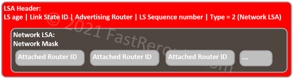
Network LSA
This LSA describes a multi-access network. Designated Router (DR) generates this LSA and lists all attached OSPF routers on the segment with which it formed an adjacency.
Link State ID in the header is DR’s IP address on the network. The mask is carried as a field with LSA, which makes it possible to identify the network address.
OSPF Packets
Earlier we have explored how OSPF sees the network, how routers describe their links and networks by generating LSAs that are flooded through the area. We also discussed how two routers synchronize their databases by becoming adjacent.
This section provides an overview of different types of packets that OSPF uses to distribute LSAs. Hello packet was introduced in the “Neighbors and Adjacencies” section. Figures 9 to 12 show the remaining types of OSPF packets.
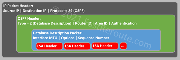
Database Description packets are used during the Database Exchange process. The packet has fields describing interface MTU, various options controlling database exchange process, and sequence numbers. The payload consists of LSA headers, which format we reviewed in the previous section.
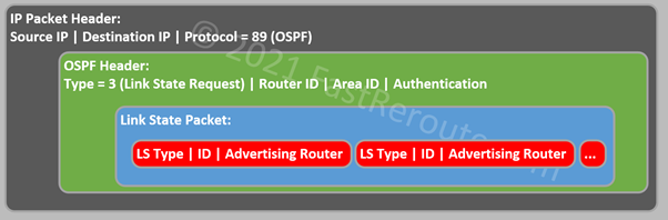
The next packet is the Link State Request packet. A router learns missing LSAs from received Database Description packets. To request those LSAs, the router sends a Link State Request packet which contains enough information to identify the LSA. These fields are LS Type, ID, and Advertising Router. The other LSA header fields, such as LS Age and LS Sequence Number, are not included. This means that the router is requesting the most recent version of LSA and not for the specific instance of LSA.
The next 2 packets are Link State Update and Acknowledgement packets. These are used to reliably flood LSAs throughout the network. Link State Update carries a list of full LSAs with their headers.
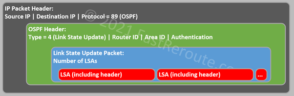
Link State Acknowledgement packet is used to explicitly confirm the receipt of a Link State Update packet.
Let’s finalize the configuration of our sample network and review different diagnostic commands.
OSPF Configuration and show commands
In this section, we will enable OSPF on different types of network interfaces using the sample topology we used earlier.
Point-to-Point Interfaces
Let’s enable OSPF between X, A, and B. In this topology, a Layer 3 LAN switch X connects to two WAN routers (A and B), which are also connected to each other.
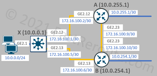
Switch X configuration is shown in the listing below.
X(config)#router ospf 100
X(config-router)#network 172.16.100.0 0.0.0.3 area 0
X(config-router)#network 172.16.100.4 0.0.0.3 area 0
X(config-router)#network 10.0.0.0 0.0.0.255 area 0
network command’s purpose is to identify interfaces that will have OSPF running and which area they will be placed in. The command uses a wildcard mask, which reverses the logic of the subnet mask. In a wildcard mask, binary 0 means “match” and 1 means “ignore”.
As subnet masks use consecutive 1s followed by consecutive 0s, it can be easily converted to wildcard mask by subtracting mask value from 255.255.255.255. For example, the hostmask of 255.255.255.255 converts to a wildcard mask of 0.0.0.0.
It is possible to use a less specific wildcard mask with a network command to match multiple interfaces with a single statement. For example, instead of the 3 commands above, we could use “network 0.0.0.0 255.255.255.255 area 0”, which would enable OSPF on all interfaces and place them into area 0.
Some data-links technologies are physically point-to-point and some of them are not. As we use Ethernet in this topology, which, by default, is treated as a multi-access network additional OSPF command is required, as shown in the listing below:
X(config)#int Gi2.12
X(config-subif)#ip address 172.16.100.1 255.255.255.252
X(config-subif)#ip ospf network point-to-point
X(config)#int Gi2.13
X(config-subif)#ip address 172.16.100.5 255.255.255.252
X(config-subif)#ip ospf network point-to-point
There is also an alternative way to enable OSPF on interfaces available in Cisco IOS-XE. Instead of performing configuration under the OSPF process, the interface-level mode can be used. Commands in OSPF process mode are still required for global parameters, such as setting router ID. The listing below demonstrates configuration on router A, a similar configuration is also applied to router B.
A(config)#router ospf 100
A(config-router)#router-id 10.0.255.1
A(config)#interface Gi2.12
A(config-subif)#ip ospf 100 area 0
A(config-subif)#ip ospf network point-to-point
A(config)#interface Gi2.23
A(config-subif)#ip ospf 100 area 0
A(config-subif)#ip ospf network point-to-point
“show ip ospf interface” command provides relevant to OSPF interface information. The network type of both interfaces is set to point-to-point with the cost of 1.
The next important information in the output below is the OSPF timers value. Hello timer defines how often Hello messages are sent and Dead interval specifies when the router will declare another one as dead without receiving hello messages. The values are automatically selected based on the network type or can be manually configured. Timers must match between neighbors.
In the example, hello and dead intervals have default values of 10 and 40.
X#show ip ospf interface
GigabitEthernet2.12 is up, line protocol is up
  Internet Address 172.16.100.1/30, Interface ID 13, Area 0
  Attached via Network Statement
  Process ID 100, Router ID 10.0.0.1, Network Type POINT_TO_POINT, Cost: 1
  <output truncated>
  Timer intervals configured, Hello 10, Dead 40, Wait 40, Retransmit 5
  <output truncated>
  Neighbor Count is 1, Adjacent neighbor count is 1
    Adjacent with neighbor 10.0.255.1
GigabitEthernet2.13 is up, line protocol is up
  Internet Address 172.16.100.5/30, Interface ID 14, Area 0
  Attached via Network Statement
  Process ID 100, Router ID 10.0.0.1, Network Type POINT_TO_POINT, Cost: 1
  <output truncated>
  Timer intervals configured, Hello 10, Dead 40, Wait 40, Retransmit 5
  <output truncated>
  Neighbor Count is 1, Adjacent neighbor count is 1
    Adjacent with neighbor 10.0.254.1
Interfaces were added using the router process “network <x> area <y>” configuration command, and this is indicated by the “Attached via Network Statement” line.
On routers A and B we used alternative configuration on the interface – “ip ospf <x> area <y>“. On these routers “Attached via Interface Enable” would be displayed instead.
“show ip ospf neighbors” command displays information about neighbors. Neighbor ID displays Router ID, and address specifies IP address of network interface over which neighbor is reachable. On point-to-point networks, neighbors always become adjacent and should be in FULL state. Because DR and BDRs are not elected on point-to-point networks priority value of 0 is set for both neighbors.
Deadtime is a count-down timer, which starts at 40 seconds and in normal conditions will not drop below 30 seconds, as hello packets are transmitted every 10 seconds.
X#show ip ospf neighbor
Neighbor ID     Pri   State           Dead Time   Address         Interface
10.0.254.1        0   FULL/  -        00:00:34    172.16.100.6    GigabitEthernet2.13
10.0.255.1        0   FULL/  -        00:00:39    172.16.100.2    GigabitEthernet2.12
Broadcast Multi-Access Network Interfaces
Let’s now finalize the configuration of the network topology by enabling connections between WAN routers (A <> C, B <> D), and connectivity between WAN routers C, D, and a switch Z.
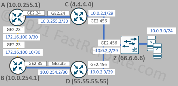
The commands used for the configuration are similar to the ones shown in the previous sections. All remaining network connections are broadcast multi-access networks, which is the default OSPF network type on Ethernet interfaces. We will omit the configuration from the previous examples that set the network type to point-to-point.
Earlier, we used interface-based configuration on routers A and B. We will apply interface-level commands for additional interfaces.
A
interface Gi2.24
 ip ospf 100 area 0

B
interface Gi2.35
 ip ospf 100 area 0
For the remaining routers, we will use the router process-based configuration. For demonstration purposes, we will set router IDs as some random values to demonstrate that these addresses are neither required to be reachable over OSPF nor belong to any of the router’s interfaces. And instead of specifying individual network statements for each interface, we will use 1 wide statement that will enable OSPF on all interfaces at once.
C
router ospf 44
 router-id 4.4.4.4
 network 0.0.0.0 255.255.255.255 area 0

D
router ospf 55
 router-id 55.55.55.55
 network 0.0.0.0 255.255.255.255 area 0

Z
router ospf 66
 router-id 66.6.6.6
 network 0.0.0.0 255.255.255.255 area 0
The next example shows “show ip ospf interface” command output on router Z. Both interfaces have OSPF network type of broadcast, which is the default for Ethernet. A manually configured router ID of 66.6.6.6 is also displayed.
Z#show ip ospf interface
GigabitEthernet2.456 is up, line protocol is up
  Internet Address 10.0.2.2/29, Interface ID 12, Area 0
  Attached via Network Statement
  Process ID 66, Router ID 66.6.6.6, Network Type BROADCAST, Cost: 1
  <output truncated>
  Transmit Delay is 1 sec, State DR, Priority 1
  Designated Router (ID) 66.6.6.6, Interface address 10.0.2.2
  Backup Designated router (ID) 55.55.55.55, Interface address 10.0.2.3
  Timer intervals configured, Hello 10, Dead 40, Wait 40, Retransmit 5
  <output truncated>
  Neighbor Count is 2, Adjacent neighbor count is 2
    Adjacent with neighbor 4.4.4.4
    Adjacent with neighbor 55.55.55.55  (Backup Designated Router)
GigabitEthernet2.2 is up, line protocol is up
  Internet Address 10.0.3.1/24, Interface ID 11, Area 0
  Attached via Network Statement
  Process ID 66, Router ID 66.6.6.6, Network Type BROADCAST, Cost: 1
  <output truncated>
  Transmit Delay is 1 sec, State DR, Priority 1
  Designated Router (ID) 66.6.6.6, Interface address 10.0.3.1
  No backup designated router on this network
  Timer intervals configured, Hello 10, Dead 40, Wait 40, Retransmit 5
  <output truncated>
  Neighbor Count is 0, Adjacent neighbor count is 0
“State DR” means that the router performs the role of the Designated Router on the network segment. Backup DR will have a state listed as BDR, and all other routers will be in DROTHER state. “Priority 1” is the default priority, so the router with the highest Router ID is elected as DR if all routers start at the same time. As the process is not preemptive, the role of DR can be performed by the router with a smaller priority or Router ID value if it starts before other routers.
Information about Designated Router and Backup Designated Routers is displayed next, followed by Hello and Dead timer settings.
The last lines of output list information about neighbors and adjacencies on the interface. Both DR and BDR become adjacent with all neighbors on the network. Routers that are neither DR nor BDR will display all routers on the segment as neighbors, however, establish adjacencies only with DR and BDR.
Link State Database
In this section, we will explore the link state database on router Z.
“show ip ospf database” command displays the content of the database. For the purpose of CCNA exam preparation, the example focuses on a single-area topology.
Z#show ip ospf database
            OSPF Router with ID (66.6.6.6) (Process ID 66)
                Router Link States (Area 0)
Link ID         ADV Router      Age         Seq#       Checksum Link count
4.4.4.4         4.4.4.4         64          0x80000014 0x00EFCE 2
10.0.0.1        10.0.0.1        1655        0x80000005 0x00F639 5
10.0.254.1      10.0.254.1      116         0x8000000A 0x00B55B 5
10.0.255.1      10.0.255.1      336         0x80000007 0x00DE3B 5
55.55.55.55     55.55.55.55     64          0x80000011 0x00B077 2
66.6.6.6        66.6.6.6        208         0x8000000C 0x0071D4 2
                Net Link States (Area 0)
Link ID         ADV Router      Age         Seq#       Checksum
10.0.2.1        4.4.4.4         209         0x80000002 0x00C617
10.0.254.1      10.0.254.1      300         0x80000001 0x00C27F
10.0.255.1      10.0.255.1      1730        0x80000002 0x00B753
Router LSA
Each router generates a Router LSA, with Link ID matching the generating router’s ID. 6 LSAs are displayed matching number of routers in our topology. To understand link count, review the previous section called “Link-State View of the Network” and Figure 6, where each outbound arrow from a router is counted as a link.
For example, let’s review in detail the content of router LSA with ID 10.0.255.1 (Router A). Below is part of Figure 6 focusing on router A.
“show ip ospf database router <router-id>” command displays detailed information about router LSA. As the link-state database is the same on all routers we can gather output on any routers in the same area. In the example below, the command is launched on router Z.
Z#show ip ospf database router 10.0.255.1
            OSPF Router with ID (66.6.6.6) (Process ID 66)
                Router Link States (Area 0)
  LS age: 142
  Options: (No TOS-capability, DC)
  LS Type: Router Links
  Link State ID: 10.0.255.1
  Advertising Router: 10.0.255.1
  LS Seq Number: 80000006
  Checksum: 0xE03A
  Length: 84
  Number of Links: 5
    Link connected to: a Transit Network
     (Link ID) Designated Router address: 10.0.255.1
     (Link Data) Router Interface address: 10.0.255.1
      Number of MTID metrics: 0
       TOS 0 Metrics: 1
    Link connected to: another Router (point-to-point)
     (Link ID) Neighboring Router ID: 10.0.254.1
     (Link Data) Router Interface address: 172.16.100.9
      Number of MTID metrics: 0
       TOS 0 Metrics: 1
    Link connected to: a Stub Network
     (Link ID) Network/subnet number: 172.16.100.8
     (Link Data) Network Mask: 255.255.255.252
      Number of MTID metrics: 0
       TOS 0 Metrics: 1
    Link connected to: another Router (point-to-point)
     (Link ID) Neighboring Router ID: 10.0.0.1
     (Link Data) Router Interface address: 172.16.100.2
      Number of MTID metrics: 0
       TOS 0 Metrics: 1
    Link connected to: a Stub Network
     (Link ID) Network/subnet number: 172.16.100.0
     (Link Data) Network Mask: 255.255.255.252
      Number of MTID metrics: 0
       TOS 0 Metrics: 1
The links in the output are shown in the following order:
- A -> N5 (A is BDR on this network, so the output displays its own IP address as DR)
- A -> B (A has point-to-point connectivity to B over N4; this is described by this link and additional link from A to N4 listed below)
- A -> N4 (numbered subnet for the point-to-point link is represented as a connection to a stub network)
- A -> X
- A -> N2
Network LSA
The next example focuses on the network LSA which represents a transit network. To display network LSA, run “show ip ospf database network <id>” command. For this example, we will use the N7 network (10.0.2.0/29) connecting routers C, D, and Z.
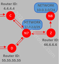
Network LSA ID matches the IP address of Designated Router (router Z) on this network and it lists router IDs of attached routers. The output shows routers Z, C, and D as attached to N7.
Z#show ip ospf database network 10.0.2.2
            OSPF Router with ID (66.6.6.6) (Process ID 66)
                Net Link States (Area 0)
  LS age: 1435
  Options: (No TOS-capability, DC)
  LS Type: Network Links
  Link State ID: 10.0.2.2 (address of Designated Router)
  Advertising Router: 66.6.6.6
  LS Seq Number: 80000002
  Checksum: 0x7325
  Length: 36
  Network Mask: /29
        Attached Router: 66.6.6.6
        Attached Router: 4.4.4.4
        Attached Router: 55.55.55.55
Network mask (/29) is also stored as part of the network LSA, which together with Link State ID represented by DR’s IP address can be used to obtain network IP prefix – 10.0.2.0/29.
Self-Test Questions
How OSPF router ID is selected if it’s not manually configured?
The highest IP address on a loopback interface. If there are no loopback interfaces, select the highest IP address assigned to a physical interface.
What OSPF uses to compare multiple paths to a destination?
By combining costs of interfaces through each path. Each interface’s cost reflects how many times its bandwidth is smaller than a reference bandwidth. If interface speed is faster or the same as the reference value, then 1 is used as cost.
What is the difference between neighbors and adjacent routers?
Neighbors are the router that can communicate with each other and have matching parameters. Adjacency is formed between neighbors for the purpose of exchanging routing information. On multi-access networks, some of the neighbors don’t establish adjacency between each other.
What are the 2 main tasks of OSPF Hello protocol?
Neighbor discovery and DR election
Explain what is router and network LSAs?
Link State Advertisement is a unit of information that is stored in each router’s Link State Database. Each router LSA represents a router and its links. Network LSA describes a transit network and lists routers connected to it.